Global Existence of Classical Solutions to a Cancer Invasion Model ()
1. Introduction
Cancer invasion is associated with the degradation of the extra cellular matrix (ECM), which is degraded by matrix degrading enzymes (MDEs) secreted by tumor cells. The degradation creates spatial gradients which direct the migration of invasive cells either via chemotaxis (cellular locomotion directed in response to a concentration gradient of the diffusible MDE) or via haptotaxis (cellular locomotion directed in response to a concentration gradient of adhesive molecules along the ECM). Chaplain and Lolas [1] proposed a PDE model of cancer invasion of tissue, which considers the competition between the following several biological mechanisms: random diffusion, chemotaxis, haptotaxis and logistic growth.
Actually, cancer invasion is a very complex process which involves many various biological mechanisms. In fact, a variety of mathematical models have been developed for various aspects of cancer invasion, and various attempts to give more biologically relevant models have been made by different people (see [2], for instance). Gatenby and Gawlinski [3] useda reaction-diffusion population competition model to study how the tumor invades the surrounding normal tissue or ECM. They suggested that tumor cells createan acidic environment that is toxic to normal tissue, and the high acidity gives rise to the death of the normal tissue, which provides space for tumor cells to proliferate and invade into the surrounding tissue. In contrast to the acid-invasion mechanism, Perumpanani and Byrne [4] found that the ECM heterogeneity affects suchinvasion. They proposed a model under the assumptions that the ECM is degraded by proteases. The proliferation of tumor cells and the remodeling of the ECM are taken into account in the Chaplain and Lolas model. Recently, Gerisch and Chaplain [5] developed a novel non-local model which incorporates cellcell adhesion and cell matrix adhesion, playing important roles in the tumor invasion process.
Very recently, Szymańka et al. [6] proposed a nonlocal model which focuses on the role of non-local kinetic terms modeling competition for space and degradation; Szymańka et al. [7] also discussed the influence of heat shock proteins on cancer invasion of tissue. The analytical results on various models of cancer invasion are mathematically interesting. Walker and Webb [8] proved the global existence solutions to the Chaplain and Anderson’s model [9]. Walker [10] also established the global existence of solutions to an age and spatiallystructured haptotaxis model, which can be regarded as an extension of the Chaplain and Anderson’s model [9]. Marciniak-Czochra and Ptashnyk recently [11] proved the uniform boundedness of solutions to the haptotaxis model [9]. Szymańka et al. [6] proved the global existence of solutions to their non-local model.
Very recently, by refining their previous techniques developed in [12]. Litcanu and Morales-Rodrigo [13] studied the asymptotic behavior of solutions to Perumpanani and Byrne’s model [4]. Paper [13], to our knowledge, is the first attempt to analytically discuss the asymptotic behavior of solutions for cancer invasion models. We should note that the cancer invasion models in [4-7,9,14] are haptotaxis only models. However, Chaplain and Lolas’ model [1] is a parabolic-ODE-parabolic-chemotaxis-haptotaxis system. The global existence and uniqueness of classical solutions to this model has been proved for  (where
  is the growth rate of cancer cells) in one space dimension (see [15]), for
  in two space dimensions (see [16]) and for large
  in three space dimensions (see [15]).We should note that the global existence is still open for small
  in three space dimensions for the parabolic-ODE-parabolic chemotaxishaptotaxis system and the parabolic-ODE-elliptic chemotaxis-haptotaxis system.
Recently, in addition to global existence and uniqueness, the uniform-in-time boundedness of solutions to a simplified parabolic-ODE-elliptic-chemotaxis-haptotaxis system has been proved for  in two space dimensions and for large
  in three space dimensions (see [17]).
This paper tries to analytically study a mathematical model of cancer invasion with . When
 , the solution Chaplain and Lolas’ model can blow up in finite time (see Section 6, [15]). However, it is obvious that the blow-up of cancer cell density in finite time is biologically irrelevant. Hence, we need to deal with the following problem: how to reasonably modify the Chaplain and Lolas’ model [1] to obtain the global existence, which is the cancer of the present paper.
This paper extends Chaplain and Lolas’ model to a parabolic-parabolic-parabolic chemotaxis-haptotaxis system, and we study the global existence and boundedness of solutions to this model. This paper organized as follows: Section 2 describes the model. Section 3 proves the local existence and uniqueness of solutions. Section 4 establishes some a priori estimates and proves the global existence.
2. Mathematical Model
The mathematical model of cancer invasion is involved in the following three physical variables: cancer cell density , ECM density
  and MDE concentration
 .
.
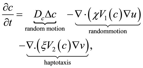
The equations describing the dynamics of each variable read as follows:
 (1)
(1)
 (2)
(2)
 (3)
(3)
where  are assumed to be positive constants and
  and
and  are the density-dependent chemotactic and haptotactic sensitivity functions, respectively.
In Equation (1), the migration of cancer cells is assumed to be governed by random motion, chemotaxis and haptotaxis. In Equation (2) is assumed that ECM has random motion and its degradation by MDEs upon contact; for simplicity, we assume that no remodeling of the ECM takes place, as done in [15,18]. Since random motion ECM is so small hence we assume that Dv is small positive constant. In Equation (3), the MDE concentration is assumed to be influenced by diffusion, production and decay; specifically, MDE is produced by cancer cells, diffuses throughout ECM, and undergoes decay through simple degradation. We shall consider the system (1)-(3) in a bounded domain 
For any  we set


To close the system of equations, we need to impose boundary and initial conditions.
Boundary conditions:
The boundary conditions are represented by the following equalities:
 (4)
(4)
where n is the our ward normal vector to ∂Ω.
Initial conditions: We prescribe the initial data
 (5)
(5)
Throughout this paper we will assume that
 (6)
(6)
 is Lipschitz continuous, (7)
where i = 1, 2 and
 (8)
(8)
In Chaplain and Lolas’ original model [1], it is assumed that  and
and  (where
  and
and  are some positive constants). For this choice of
  and
and  although the assumptions (6)- (8) are satisfied but we would like to slightly modify the choice of
  such that the modified model has a unique global solution. To this end, in addition to the assumptions (6)-(8), we will assume that
 (9)
(9)
 (10)
(10)
For example, we may take 
 and
and  (
( are small positive constants ). Clearly
  as
as  as
as  and
and  For this choiceof
 , and
, and , the assumptions (6)-(10) are satisfied. Another choice of
  and
and  satisfying (9) is that
  for
for  which has a clear biologically relevant interpretation: the cancer cells stop to accumulate at a given point of the tumor tissue after their density attains a maximal density
  A similar assumption for a prey taxis sensitivity function was made in [19].
In next section we will prove the local existence and uniqueness of a solution for the system (1)-(5) by a fixed point argument.
3. Local Existence and Uniqueness
Throughout this paper we assume that
 (11)
(11)
For brevity we set
 (12)
(12)
For notations’ convenience, in what follows we denote various constants which are independent of T by A0, whereas we denote various constants which depend on T by A .The constants A0 and A may be different from line to line.
In the following, under the assumptions (6)-(8) and (11), we shall prove that the system (1)-(5) has a unique local (in time) smooth solution.
Theorem 3.1. Under the assumptions (6)-(8), there existsa unique solution  of the system (1)-(5) for some small
  which depends on

Proof. We shall prove the local existence by a fixed point argument. We introduce the Banach space X of the vector function U (defined in (12)) with norm

and a subset

where

Given any  we define a corresponding.
Function  by
by , where
  satisfies the equations
 (13)
(13)
 (14)
(14)
 (15)
(15)
 (16)
(16)
 (17)
(17)
 (18)
(18)
 (19)
(19)
 (20)
(20)
 (21)
(21)
where
 (22)
(22)
We first consider the linear parabolic (13)-(15). By (8), (11) and the parabolic Schauder theory (for example, see [20]) there exists a unique solution , and
, and
 (23)
(23)
Similarly, from  (11) and the parabolic Schauder theory, problem (16)-(18) has a unique solution
  satisfying
 (24)
(24)
We now turn to the linear parabolic problem (19)-(21). Using  (23) and (24) and noting
  and
and  are Lipschitz continuous, we have
 (25)
(25)
Hence, by Schauder theory as before, the problem (19)- (21) admits a unique solution  satisfying
 (26)
(26)
We conclude from (23), (24) and (26) that
 (27)
(27)
By direct calculations, we obtain

where  If we further take T sufficiently small, then by (27)

Hence,  , i.e.
  maps
maps  into itself. We next show that
  is a contraction mapping. Take
  and set
  and
and . setting

We derive from (13) that

where

Hence, since  Schauder theory yields
 (28)
(28)
Similarly, we derive from (16) and 
that
 (29)
(29)
We next turn to the equation for :
:
 (30)
(30)
where

Noting  and
and  are Lipschitz continuous and using (6), (7), (27), (28) and (29), we have

By Schauder theory, since 
 (31)
(31)
Combining this with (28) and (29), we get

Nothing  and proceeding as before, we have
 (32)
(32)
Taking T small such that  we conclude from (32) that F is a contraction in
 . By the contraction mapping theorem F has a unique fixed point
  in
in  which is the unique solution of (1)-(5).
4. A Priori Estimates and Global Existence
To continue the local solution established in the above section to all t > 0 we need to establish some a priori estimates. Throughout this section, in addition to the assumptions (6)-(8) and (11) we assume that the assumptions (9) and (10) hold.
Noting  and
and  and using the maximum principle, we easily prove the following lemma.
Lemma 4.1. Assume that  is a solution to (1)-(5), then
 (33)
(33)
Lemma 4.2. Assume that  is a solution to (1)-(5) then for
 , we have
 (34)
(34)
 (35)
(35)
 (36)
(36)
Proof. For , we derive from
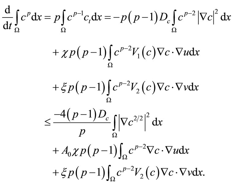 (37)
(37)
We now consider the integral . By Equation (3) and the parabolic
  estimate [20] we have
 (38)
(38)
In particular,
 (39)
(39)
Multiplying Equation (3) by  and integrating in
 , we obtain

And there for, by Young’s inequality and estimate (39), we have
 (40)
(40)
Also, by Equation (2) and the parabolic  estimate we have
 (41)
(41)
In particular,
 (42)
(42)
By (9), Young’s inequality and estimate (42)
 (43)
(43)
Integrating with respect to t on both sides (37), noting (11) and using estimates (40) and (43) and taking  sufficiently small, we obtain

Gronwall’s lemma yields
 (44)
(44)
Now, by (39) and (44) we have
 (45)
(45)
This completes the proof of lemma 4.2.
In the following result we obtaina better bound of c, a —bound. Let p > 1 and define
 , with domain
  For each
 define the sectorial operator
  (see [21]) and
 with the norm
Lemma 4.3. Let  then for
  where
where , we have
 (46)
(46)
Proof. We have that

and so
 (47)
(47)
By [21] (Theorem 1.4.3) and (11)
 (48)
(48)
and, by (34),
 (49)
(49)
where . Moreover, by [22] (Lemma 2.1), (9), (35) and (36), we obtain
 (50)
(50)
where 
Inserting (48)-(50) into (47) and noting 
and , we obtain

for all 
This completes the proof of lemma 4.3.
Lemma 4.4. We have that
 (51)
(51)
Proof. Let  we have by [21] (Theorem 1.6.1) that

Thanks to lemma 4.3 we have that

Moreover, the local existence Theorem yields  for
for 
Therefore

This completes the proof of Lemma 4.4.
Lemma 4.5. We have that
 (52)
(52)
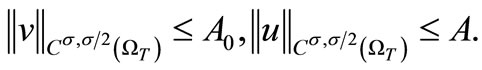
Proof. By the Sobolev embedding theorem (see [20], (Lemma 3.3, p. 80)), if we take p sufficiently large, then (35) and (36) yields
 (53)
(53)
and therefore
 (54)
(54)
By (7) and (51), we have
 . (55)
Now, Equation (1) can be rewritten as

where
 (56)
(56)
 (57)
(57)
By (9), (35), (36), (53) and (55). These, along with (11) and the parabolic  estimate, yield the estimate (52).
Lemma 4.6. Assume that  is a solution to (1)-(5), then
 (58)
(58)
Proof. By (52) and the Sobolev embedding theorem (taking p large),
 (59)
(59)
Also, (35), (36) and the Sobolev embedding theorem (taking p large) yield
 (60)
(60)
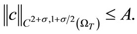
Now, from (3), (11), (59) and the parabolic Schauder estimates we have
 (61)
(61)
Also, the parabolic Schauder estimates yield
 (62)
(62)
Finally, we conclude from (61) and (62) that

Hence, by the parabolic Schauder estimates, we obtain
 (63)
(63)
This completes the proof of Lemma 4.6.
With a priori estimate (58), we can extend the local classical solution established in Theorem 3.1 to all , as done in [15]. Namely we have Theorem 4.7. There exists a unique global solution
  of the system (1)-(5) for any given
 .
.
NOTES