Transient Stability Analysis of 33 KV Transmission Network of Egi Community, Nigeria

Promise Elechi, Christopher Okwuchukwu Ahiakwo, Ugochukwu Nureedin Okwu

Department of Electrical/Electronic Engineering, Rivers State University, Port Harcourt, Nigeria.

DOI: 10.4236/jpee.2020.83002                

Abstract

Transient analysis of 33 KV power transmission line stability of Egi communi-ty is considered in this research work with the aim of reducing the frequency of fault occurrence and voltage collapse in the network. The supply is taken from Egi generating station located at Total Nigeria Limited Gas Plant Obite at voltage level of 33 KV to Egi communities. This work focuses on the transient nature of network stability since transient fault is the most dangerous in elec-trical systems. The swinging of the generator rotor in the event of transient three-phase short circuit fault can be monitored by the circuit breakers and the protective relays which causes mal-functioning of the circuit breakers and pro-tective relays leading to abnormal behavior of the network. Therefore, data obtained from the power station were used as a case study of Independent Power Producer (IPP) in Nigeria. For investigation of the power angle, angular velocity, rotor angle differential changes, and angular velocity differential changes, an electrical transient analyzer tool was employed (ETap version 16.00) for circuit breaker and protective relay time setting of (0.00, 0.05, 0.10, 0.15, 0.20, 0.25, 0.30, 0.35, 0.40, 0.45, 0.50, 0.55, 0.60). The work used the Trapezoidal numerical technique for data analysis. The graphs were plotted using Matlab R2015a and the results obtained showed that when a symmetrical three-phase short circuit fault occur at one or any of the feeders, the fault must be cleared as quick as possible through the coordination of the circuit breakers and protective relays. For this research work, 17 cycles corresponding to relay time setting of t = 0.34 s were recommended and at each cycle, changes in time with respect to changes in rotor angle, angular velocity, rotor differential and angular velocity differential were calculated on the power network simultaneously. The results demonstrated that the Trapezoidal method is numerically stable, accurate and has faster respond time when compared to Modified Euler and swing equation techniques in event of fault occurrence in network.

Keywords

Rotor Angle, Transient Stability, Swing Equation, Angular Speed, Differential Changes, Trapezoidal Rule, Fault Clearing Time, Critical Clearing Time

1. Introduction

Electrical energy demand in Egi community is continuously increasing each year in both the domestic and industrial sectors as most villages are hooked up to Egi network and industries and businesses are established to meet the demand of the teeming population. The establishment of Egi Gas Turbines by Total Exploration and Production Nigeria Limited (TEPNG) to supply electrical power to the host communities has improved the economic activities of the people; hence electrical energy will continue to be the single most important energy in these communities as it plays a crucial role in the development of any society. To distribute electrical power from Egi Gas Turbine to the neighboring communities, transmission and distribution lines were built and they are far away from the power station and from each other. The power station output is connected and transmitted through the Egi Transmission and Distribution Network (ETDN) to the respective communities [1].

The interconnected electric power network (ETDN) present various challenges to Total Exploration and Production Nigeria Limited, the operator of the power station, these problems are due to inherent nature of power system through planning, construction, operation and control. One of these challenges is transient stability or voltage stability. The Transient instability in Egi transmission network is caused by a number of factors which ranges from atmospheric phenomenon like lightening, solar fares, geomagnetic interference, sudden addition of inductive load, switching load ON and OFF, switching of power lines especially during repairs, interruption of fault current by breakers etc. The instability in the power network had led to the collapse of the feeders of Egi Gas Turbine on several occasions [1] [2].

Steady and efficient electricity supply from TEPNG resulted in massive industrialization within the Egi communities, as more welding shops, salon shops, grinding shops and businesses are evolving everyday which translates to more inductive load on the network, the resultant effect is that by 2007, the network could no longer be synchronized. This led to voltage instability in the system which results to constant load shedding and delivering of poor power supply to the communities [2]. Generally, transient instability is a major challenge in power system operation and control. At present, feeders 1 and 2 have just been reinstalled into operation which collapsed as a result of instability in the network. In order to reduce the frequency and duration of load shedding, a total of 3 MW was formally transferred to the Rivers State Generation Plant at Omoku. It is on this basis that the following problems were identified:

1) Complete collapse of feeder 1 and 2 of Egi Gas Turbines as a result of instability in the network.

2) Continuous addition of inductive load on the system by establishment of welding and fabrication workshops, wood sawing workshops, grinding shops and palm/kernel mills resulting to instability in the network.

3) Increasing demand of power for domestic use due to influx of population and expansion of the communities by building new houses which add more load to the network causing system instability.

4) Establishment of high local micro businesses like salon and barbing shops, frozen fish/meat shops, cooled drink and restaurants etc. are also on the increase which add load that affect system stability.

5) The current load demand exceeds the power generation capacity hence leading to total system collapse.

The existing total load consumption would continue to increase, hence, the need to carry out forecast study for effective operation of the plant [2]. For stability of power system, the fault clearing time (FCT) and the critical clearing time (CCT) has to be determined and specified [3].

2. Methodology

2.1. Materials and Method

This work investigated the behaviour of transient stability of 33 KV transmission network of Egi community with emphasis on the behaviour of 9.455 MVA synchronous generators after a large disturbance on the power network. The generation, transmission and distribution data were collected and analyzed. The data of the power network collected and the results generated were analyzed. An Etap analyzer was used and results were generated. The changes in time (t) against changes in power angle and changes in time (t) against changes in angular velocity were investigated using analytical tool. The swing equation model and Trapezoidal rule were used to determine the accelerating power of the synchronous generators when the load was suddenly removed. The coordination of the network relays and the circuit breakers is crucial to the stability of power network; the relays are programmed to sense the fault and transmitted to the circuit breakers to isolate any faulty part of the system to avoid system collapse. The faster these sensors act in micro-second, the more stable the network. Electrical fault in power network can be categories into three (3) distinct parts namely, the pre-fault condition, fault condition and post fault condition [3].

Electrical faults in power systems are non-linear in nature therefore requires non-linear solutions. Figure 1 represent the equivalent machine model of a synchronous generator, the excitation voltage E' is behind the transient reactance ${E^{\prime }}_d$. This research work will adopt the application of implicit method using Trapezoidal Rule in resolving transient stability of 33 KV transmission network of Egi community, Nigeria and compare it with Modified Euler and the nominal Swing equation techniques. Figure 2 is the power transfer curve. Figure 3 is the single line diagram of the power supply from Egi gas turbine to the communities. Figure 4 is the simulated network from Egi gas turbine to 33 Kv transmissions and distribution network. Figure 5 is the graph of incremental changes of machine rotor angle against time, while Figure 6 is comparison of changes in machine rotor of Swing, Modified Euler and Trapezoidal methods against changes in time. Figure 7 is the simulated swing curve of the rotor angle of the case study.

In determining the transient stability of power system, the active power transferred by generator plays important role since the stability of the system is influenced by the angle stability of the generators which are connected to a complex network of inter-connected power system [3] and [4].

In normal operating condition, the relative position of the rotor axis and the stator magnetic field are fixed [5]. The angle between the rotor axis and the stator field is known as the torque angle, if the loading of the generator is large, the torque angle δ will invariably be large [5]. If a load torque T_L is applied suddenly, the generator may lose synchronism (fall out of step) even if the load torque is less than maximum torque δ_max the generator can develop. The maximum value of the load torque that can be applied suddenly to the generator without the generator losing synchronism can be obtain from the dynamic behavior of the synchronous generator.

Let consider an unloaded synchronous generator connected to a power system, if losses are neglected, the torque angle δ_g is zero. If a load torque δ_L is suddenly applied to the shaft of the synchronous generator, the generator speed slows down and the torque angle δ_g increases. As the torque angle δ_g increases, the generator develops more torque δ_g to meet the load torque δ_L. The torque angle δ_g reaches the value of the load torque δ_L at which the load torque δ_L equals the torque angle δ_g of the generator as shown in Figure 2.

However due to inertia the torque angle δ_g increases beyond the load torque δ_L and the generator develops more torque than required for the load. The deceleration decreases and the torque angle δ_g reaches a maximum value δ_max and then swings back. The torque angle δ_g oscillates around the load angle δ_L, due to damping in the system, the torque angle will settle down to the required value of load angle ${{\delta }^{\prime }}_L$. The oscillation of the torque angle δ_g last for several cycles and it can be assumed that Figure 1 shows satisfactory representation of the electrical system.

The oscillation in the torque angle δ_g as a function of time can be obtained in solving the differential equation that describes the behavior of the system [5] and [6].

The excitation voltage behind the transient reactant of a synchronous generator is expressed as:

${E^{\prime }}_g=V+J{X^{\prime }}_{d}I$ (1)

Figure 1. Equivalent machine model [4].

Figure 2. Power transfer curve [4].

Figure 3. Single-line diagram of power supply from Egi station to the communities.

where ${E^{\prime }}_g$ = excitation voltage;

V = bus voltage;

${X^{\prime }}_d$ = transient reactance [5] and [6].

The total reactance during the period of transient stability is the addition of transformer reactance $X_t$, the line reactance $X_l$ and the transient reactance ${X^{\prime }}_d$,

$X_{eq}=X_l+X_t+{X^{\prime }}_d$ (2)

where $X_l$ = Line reactance;

$X_t$ = transformer reactance;

${X^{\prime }}_d$ = transient reactance [3] and [7].

The equation which describe the relative change of position of the rotor (the torque angle) with respect to the stator as a function of time is the swing equation which can be expressed in terms of toque or power of the machine, hence,

$P_a=P_s+P_e$ (3)

$P_a$ = Accelerating power;

$P_s$ = Mechanical power;

$P_e$ = Eletromagnetic power [5].

The electromagnetic or electrical power is equivalent to the product of the generator voltage, the electromagnetic voltage developed by the generator, the sine of the torque angle and the reciprocal of generator reactance.

$P_e=\frac{V_g{V}_m}{X_g}\sin {\delta }_g$ (4)

$V_g$ = generator voltage;

$V_m$ = Electromagnetic voltage developed by generator;

$X_g$ = Generator reactance;

${\delta }_g$ = generator torque angle [7].

The shaft power (mechanical power) is the power transferred or developed by shaft of the generator due to load and is given by

$P_s=\frac{E_g{E}_l}{X_d}\sin {\delta }_l$ (5)

$E_g$ = Generator voltage;

$E_l$ = Load voltage;

$X_d$ = Line reactance;

${\delta }_l$ = Load torque [7].

Appling the principle of rotation, the swing equation that relates the inertia of prime mover and generator is:

$Kj\frac{{\text{d}}^2\delta }{\text{d}{t}^2}$

where j = moment of inertia of prime mover and generator;

Kj = inertia constant of machine [8].

The power balance equation of a synchronous rotating generator can be expressed as,

$\frac{E_g{E}_l}{X_{eq}}\sin {\delta }_l=K_j\frac{{\text{d}}^2\delta }{\text{d}{t}^2}+\frac{V_g{V}_m}{X_{eq.}}\sin {\delta }_g$

$P_{\max }\sin {\delta }_l=K_d\frac{\text{d}\delta }{\text{d}t}+K_j\frac{\text{d}{\delta }^2}{\text{d}{t}^2}$ (6)

This is known as the swing equation and the trapezoidal rule is used to evaluate the load angle ( ${\delta }_l$ ).

2.2. Bus Data

The network bus loading in the case study is the maximum and minimum load range from Egi Gas turbine data base. The generator and network data used for this work are presented in Tables 1-4.

Table 1. Network parameters.

Table 2. Generation system parameters (Egi Gas Turbine).

Table 3. Bus loading for the transmission network.

Table 4. Study case designation, (Egi Gas Turbine).

2.3. Calculation of Line Network Parameters

Using MVA base of 20 MVA

$P_e=\frac{28.4}{20}={1.42}_{p.u}$

$P_m=\frac{31.6}{20}={1.58}_{p.u}$

Reactance:

$X_{eq}$ = generator reactance + line reactance + transformer reactance [3] and [5].

$X_{eq}={0.19}_{p.u}+{0.013}_{p.u}+{0.03}_{p.u}$

$X_{eq}={0.35}_{p.u}$

Real Power (S) [8]:

$S=\frac{P_e}{P_f}\angle {\cos }^{-1}(\varnothing )$ (7)

where $P_f=\varnothing =0.8$ [9].

$S=\frac{1.42}{0.8}\angle {\cos }^{-1}\left(0.8\right)=1.775\angle 36.87$

Current:

$I=\frac{S^{*}}{V^{*}}=\frac{1.775\angle -36.87}{1.0\angle 0}$

$I=1.775\angle -36.87$

Excitation Voltage [5] and [6]:

${E^{\prime }}_g=V+J{X^{\prime }}_{d}I$

Therefore, we have:

${E^{\prime }}_g=1\angle 0+\left(j0.35\right)\left(1.775\angle -36.87\right)$

${E^{\prime }}_g=1+j0+\left(0.35\angle 90\right)\left(1.775\angle -36.87\right)$

${E^{\prime }}_g=1+j0+0.3728+j0.4970$

${E^{\prime }}_g=1.3728+j0.4970$

${E^{\prime }}_g={1.3728}_{p.u}$

Therefore, we have the initial operating condition as follows [8]:

$H=5.673\text{p}\text{.u}$

${\omega }_0={\omega }_L=2\pi f_o=2\times \pi \times 50=314.1593\text{rad}/\text{sec}$

${\delta }_0={\delta }_L={23.2}^{\circ }$

$1\text{rad}={57.32}^{\circ }$

Therefore, ${23.2}^{\circ }\text{in}\text{rad}=\frac{{23.2}^{\circ }}{{57.32}^{\circ }}=0.4047\text{rad}$ [6].

2.4. Application of Swing Equation Technique to Transient Stability

Applying the values into the swing equation technique [7]:

$\frac{H{d}^2\delta }{\pi fd{t}^2}=P_m-P_e$ (8)

where $\frac{H{d}^2\delta }{\pi fd{t}^2}=P_a=\text{accelerating}\text{power}$ [7] and [8].

Substituting into Equation (8) we have:

$\frac{5.673}{\pi \times 50}\frac{{\text{d}}^2\delta }{\text{d}{t}^2}=\left(1.58-0\right)$ (during fault)

$\frac{5.673}{\pi \times 50}\frac{{\text{d}}^2\delta }{\text{d}{t}^2}=1.58$

$\frac{{\text{d}}^2\delta }{\text{d}{t}^2}=1.58\times \frac{\pi \times 50}{5.673}$

Integrating both sides:

$\frac{\text{d}\delta }{\text{d}t}={\displaystyle \int \frac{\pi \times 50}{5.673}\text{d}t}\times 1.58$

$\frac{\text{d}\delta }{\text{d}t}={{\displaystyle \int }}^{\text{}}\frac{\pi \times 50}{5.673}\text{d}t+0$

Integrating the second time:

$\text{d}\delta \left(t\right)=\frac{\pi \times 50}{11.346}{t}^2+{\delta }_0$

$\text{d}\delta \left(t\right)=\frac{\pi \times 50}{11.346}{t}^2+0.4047$

$\delta \left(t\right)=\frac{\pi \times 50}{11.346}{t}^2+0.4047$

The iteration is repeated for thirtieth cycles.

2.5. Application of Trapezoidal Rule to Transient Stability Analysis

Applying the Trapezoidal rule and the two mechanical equations that describe the rotor dynamics, the trapezoidal rule can be investigated for thirtieth cycles as follow [9]:

${\delta }_{n+1}={\delta }_L+\frac{\Delta t}{2}\left(\frac{\text{d}{\delta }_n}{\text{d}t}+\frac{\text{d}{\delta }_{n+1}}{\text{d}t}\right)$ (10)

${\omega }_{n+1}={\omega }_L+\frac{\Delta t}{2}\left(\frac{\text{d}{\omega }_n}{\text{d}t}+\frac{\text{d}{\omega }_{n+1}}{\text{d}t}\right)$ (11)

where,

${\delta }_{n+1}$ = machine rotor angle evaluated at n + 1;

${\delta }_L$ = Latest rotor angle;

$\frac{\text{d}{\delta }_n}{\text{d}t}$ = differential rotor angle evaluated at n;

$\frac{\text{d}{\delta }_{n+1}}{\text{d}t}$ = differential rotor angle evaluated at n + 1;

${\omega }_{n+1}$ = angular speed evaluated at n + 1;

${\omega }_L$ = Latest angular speed;

$\frac{\text{d}{\omega }_n}{\text{d}t}$ = differential angular speed evaluated at n;

$\frac{\text{d}{\omega }_{n+1}}{\text{d}t}$ = differential angular speed evaluated at n + 1;

$\Delta t=0.02\text{s}$, interval between cycles and is constant throughout the period of iteration.

$\frac{\text{d}{\delta }_n}{\text{d}t}=\left({\omega }_L-2\pi f_o\right)$ [9] and [10]. (12)

$2\pi f_o$ = Synchronous speed

$\frac{\text{d}{\omega }_n}{\text{d}t}=\frac{1}{M}\left(P_m-P_e\right)$ [9]

where $M=\frac{H}{\pi f_o}$

$\frac{\text{d}{\omega }_n}{\text{d}t}=\frac{1}{\frac{H}{\pi f_o}}\left(P_m-P_e\right)$

$\frac{\text{d}{\omega }_n}{\text{d}t}=\frac{50\pi }{H}\left(P_m-P_e\right)$ (13)

where H = inertia constant;

$P_m$ = mechanical power;

$P_e$ = electrical power.

During fault, $P_e=0$ [9] [10] and [11].

Iteration at t = 0

Evaluation of $\left(\frac{\text{d}\delta }{\text{d}t},\frac{\text{d}\omega }{\text{d}t},\delta ,\omega \right)$

Substituting in Equation (12)

$\frac{\text{d}{\delta }_0}{\text{d}t}=\left({\omega }_L-2\pi f_o\right)$

$\frac{\text{d}{\delta }_0}{\text{d}t}=\left({\omega }_L-314.1593\right)$

Here ${\omega }_L=314.1593$,

$\frac{\text{d}{\delta }_0}{\text{d}t}=314.1593-314.1593$

$\frac{\text{d}{\delta }_0}{\text{d}t}=0$

Again, from Equation (13)

$\frac{\text{d}{\omega }_0}{\text{d}t}=\frac{50\pi }{H}\left(P_m-P_e\right)$

$\frac{\text{d}{\omega }_0}{\text{d}t}=\frac{50\times \frac{22}{7}}{11.346}\left(1.58-0\right)$

$\frac{\text{d}{\omega }_0}{\text{d}t}=13.8501\left(1.58-0\right)$

$\frac{\text{d}{\omega }_0}{\text{d}t}=21.8831$

Applying Trapezoidal rule at 0

$\delta \left(0\right)={\delta }_L+\frac{\Delta t}{2}\left(\frac{\text{d}{\delta }_0}{\text{d}t}\right)$

$\delta \left(0\right)=0.4047+\frac{0}{2}(0)$

$\delta \left(0\right)=0.4047\text{rad}={23.2}^{\circ }$

$\omega \left(0\right)={\omega }_L+\frac{\Delta t}{2}\left(\frac{\text{d}{\omega }_0}{\text{d}t}\right)$

$\omega \left(0\right)=314.1593+\frac{0}{2}\left(21.8831\right)$

$\omega \left(0\right)=314.1593\text{rad}/\text{sec}$

$\left[\begin{array}{l}\delta \left(0\right)=0.4047\text{rad}={23.2}^{\circ }\\ \omega \left(0\right)=314.1593\text{rad}/\text{sec}\end{array}\right]$

${\delta }_L=0.4047\text{rad}$

${\omega }_L=314.1593\text{rad}/\text{sec}$

The iteration is repeated for thirtieth cycles.

Calculation of Critical Clearing Time (CCT)

Critical clearing time, $t_{cr}$ [9]:

$t_{cr}=\sqrt{\left({\delta }_{cr}-{\delta }_0\right)\cdot \frac{4H}{{\omega }_s{P}_m}}$ [12] (14)

where,

$t_{cr}$ = critical clearing time [6];

${\delta }_{cr}$ = critical clearing angle = 89.63˚ = 1.5637 rad;

${\delta }_0$ = initial angle = 23.2˚ = 0.4047 rad;

${\omega }_s$ = synchronous frequency = 314.1593 rad/sec;

$P_m$ = mechanical power or shaft power = 31.6 MW;

H = inertia constant of generators = 3 MJ/MVA.

Substituting,

$t_{cr}=\sqrt{\left(1.5637-0.4047\right)\times \frac{4\times 3}{314.1593\times 31.6}}$

$t_{cr}=0.037\text{s}\approx 0.04\text{s}$

It implies that for effective fault clearing operation of the relay coordination and circuit breakers, the relay setting time should be 0.04 s. This will clear the three-phase fault as fast as possible for the network to be in synchronism with the machine to avert system collapse.

3. Results and Discussion

The results of the rotor angle and the angular velocity are represented for detail analysis of the power network. The results show the inherent nature of the network variables when subjected to external disturbance and occurrence of fault on any part of the network. The results are therefore presented as follows (Figures 4-7 and Tables 5-7).

The graph of Figure 5 shows the characteristics behavior of the machine rotor angle (δ) of the Trapezoidal method against time (t). The machine rotor angle in degree gradually increased from when the fault was initiated at t = 0 and rotor angle of 23.2˚ up to maximum allowable stability angle of 90˚ and continued up to 161.44˚ at t = 0.6 s. The network is very unstable and cannot be synchronized because the rotor angle keeps increasing even when the speed has reduced. The increase in machine rotor angle beyond 90˚ is an indication of instability in the network which will trigger loss of synchronization if corrective action is not taken. It is shown that the fault was cleared at the seventeenth cycles at t = 0.34 s (FCT) and rotor angle of 85.05˚, but the machine rotor angle continues to increase up to 161.44˚, even when the angular speed has decreased suggesting that the machine and the network is unstable and the generator is running under heavy loads which will lead to system collapse. Table 6 shows the incremental time against the rotor angle for swing, modified Euler and trapezoidal methods.

Figure 4. Simulated Network from Egi Gas Turbine to 33 KV Transmission network.

Table 5. Incremental time (t) with changes in rotor angle (δ) for trapezoidal method.

Figure 5. Graph of machine rotor angle (δ) against time for trapezoidal method.

3.1. Analysis of the Simulated Case

Figure 6 is the presentation of the machine rotor angle analysis in the case study at different operating time. Rotor angle (rd1) represent the case of fault which lasted for several time resulting to instability in the system, (rd2) is the rotor angle in the case of fault but was cleared very quick after 1.5 cycles which enable

Table 6. Incremental time (t) against rotor angle (δ) for swing, modified euler & trapezoidal methods.

Figure 6. Presentation of comparison of swing, modified euler and trapezoidal curves.

the rotor angle to returned to stability, (rd3) is the rotor angle in the case of fault up to 3.5 cycles which was cleared for the network to returned to stability while (rd4) is the rotor angle at fault up to 5.5 cycles which lasted for much longer time to be cleared before the network settle to stability

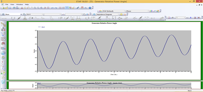
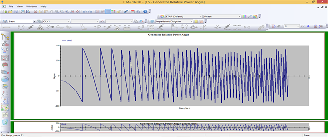
Appendix B1 shows when a three-phase fault occurred at feeder 1 and the result of the simulation present the swinging of generator rotor angle which indicate unstable state. The swing curves show that the fault region is near to generator. Appendix B2 shows generator rotor angle when the three-phase fault was cleared at 1.5 cycles and the network returned to stability region.

Appendix B3 shows generator rotor angle with fault cleared at 5.5 cycles, initially the network was unstable at the occurrence of the fault at t = 0, but

Table 7. Changes in time (t) against changes in rotor angle (δ₁, δ₂, δ₃, δ₄) obtained from simulation.

Figure 7. Simulated swing curve of rotor angle against time (t).

through the coordination action of relays and circuit breakers, the network was immediately brought to synchronism at 5.5 cycles after clearing the fault.

4. Conclusion and Recommendations

4.1. Conclusion

This research work described the behavior of transient stability of 33 Kv transmission network of Egi community with emphasis on the behavior of 9.455 MVA synchronous generators after a large disturbance on the power network. The generation, transmission and distribution data were collected and analyzed. The data of the power network collected and the results generated were analyzed. An Etap analyzer was used and results were generated. The changes in time (t) against changes in power angle (δ) and changes in time (t) against changes in angular velocity (ω) were investigated using analytical tool. The swing equation model and Trapezoidal rule were used to determine the accelerating power of the synchronous generators when the load was suddenly removed. Stability could not be obtained even when network fault was cleared at t = 17 cycles = 0.34 s (FCT) and power angle of 87.05˚, above 17 cycles the swinging caused by network disturbance causes network instability. The results of the swinging curves and load flow were also presented at the appendices.

4.2. Recommendations

Successful operation of power system plants depends on the ability of the power engineers to adopt and apply the recommendations resulting from transient and load flow stability studies to prevent network collapse. If these studies are taken seriously, it will prevent total network break down and collapses.

The following points should be noted from the investigation and study of the transient stability analysis of 33KVEgi transmission network for considerations:

1) Continuous evaluation of reactive power and the power angle (machine rotor angle).

2) Fast and high-speed operation of protective relays and circuit breakers with fault clearing time set at t = 0.04s.

3) Expansion of the generating units to meet the load demand.

4) Installation of time-synchronizing phasor measurement units to monitor network coordination.

5) Minimization of transfer reactance to increase power.

Appendices

Appendix B1

Appendix B2

Appendix B3

Conflicts of Interest

The authors declare no conflicts of interest regarding the publication of this paper.

References

[1]	Rapu, I. and Okeke, C. (2018) Presentation on Egi/Rivers State Ministry of Power Interface.
[2]	Total Nigeria Maintenance Report (2019) JV-Field Operations-OML 58 Maintenance Report. Total Nigeria, Electrical Methods, JV Operation.
[3]	Ahiakwo, C.O., Braide, S.L. and Aghaukwu, N.C. (2019) Analysis of 232 KV Power Transmission Stability in a Developing Nation. American Journal of Engineering Research, 8, 124-132.
[4]	Obe, E.S. (2009) Lecture Note on Synchronous Machines.
[5]	Duncan, G. (2008) Power System Analysis and Design. 2nd Edition, Wiley Publishers, New York.
[6]	Gupta (2005) Power System Engineering. 2nd Edition, S. Chand Publishers, India.
[7]	Omorogiuwa, E. and Elechi, P. (2015) Impact of Distributed Generation Placement on Stability of Power Network in Nigeria. IOSR Journal of Electrical and Electronics Engineering, 10, 61-69.
[8]	Omorogiuwa, E. and Elechi, P. (2015) Economic Effects of Technical and Non- Technical Losses in Nigeria Power Transmission System. IOSR Journal of Electrical and Electronics Engineering, 10, 61-69.
[9]	Kai, S. (2018) Lecture Notes on Power System Analysis II and 3-Power System Stability.
[10]	Enemuoh, F.O. (2012) Simulation Modelling of Voltage Stability of an Interconnected Electric Power System Network.
[11]	Ghorban, A.K.M. and Mozafari, B. (2012) Impact of SVC on Transmission Lines. Electric Power and Energy System, 4, 702-709. https://doi.org/10.1016/j.ijepes.2012.04.029
[12]	Kumur, A. and Dubey, S.B. (2013) Enhancement of Transient Stability in Transmission Line Using SVC Fast Controller. International Journal of Recent Technology and Engineering, 2, 7-13.