What Are the Socio-Economic Predictors of Mortality in a Society?

Wahab Adewuyi Adejumo¹, Adetunji Raimi Tijani¹, Sheriff Adesanyaonatola²

¹Department of Insurance, the Oke-Ogun Polytechnic Saki, Oyo State, Nigeria.
²Department of Insurance, the Polytechnic Ibadan, Oyo State, Nigeria.

DOI: 10.4236/jfrm.2019.84017                

Abstract

Improvement in medical science is regarded as one of major factors that led to the constant improvement of living conditions in most of the countries with the result that mortality rate has been declining, thereby resulting in a steady increase of life expectancy which further led to creating higher financial responsibilities for pension and annuity providers. In essence, mortality forecasts are essential for predicting the future extent of population ageing, and for determining the sustainability of pension schemes and social security systems. The objective of this paper is to fit multiple regression models to measure how the various predictive variables relate to mortality. We intend to select a statistical model from the model class that best fits the data by choosing the model that has the smallest AIC value. From the analysis of our research, we found that income deprivation is the strongest independent predictor of mortality rates in a neighbourhood, though each of the variables is statistically significant at less than 5%.

Keywords

Multiple Regression, Predictive Variables, Model Selection, Income Deprivation, Relative Risk

1. Introduction

Mortality rate is an important variable in the fields of actuarial science, demography, national planning and social security administration and as a result of this, it is generally regarded as an indicator of a general welfare of a population (Cerda-Hernandez & Sikov, 2018).

During the last decades, mortality has significantly declined in most developed countries around the world, mainly due to the continuous improvement of living conditions and the evolution of medical science and technology, thereby resulting in a steady increase of life expectancy, which in turn creates higher financial responsibilities for governments, pension and annuity providers (Bozikas & Pitselis, 2019). The pension and annuity writers usually made use of the predicted mortality rates in their pricing calculations and any underestimation of the longevity risk may eventually cause a financial collapse of these companies.

More so, Longevity risk, according to Marius (2018), defined as the risk that people live longer than expected, represents an important issue for current societies. Although longevity advancements increase the productive life span and welfare of millions of individuals, there are also increasing costs for pay-as-you-go (PAYG) and defined benefits pension systems, threatening the long-term solvency of financial institutions due to increases in unanticipated future liabilities (Marius, 2018). Additionally, public health expenditures may be unnecessarily increased if unhealthy life expectancy is extended owing to general reduction in mortality rate.

In essence, mortality forecasts are essential for predicting the future extent of population ageing, and for determining the sustainability of pension schemes and social security systems (Janssen, 2018).

In one word, prediction of future mortality rates is especially useful for life insurance companies, pension consultants and annuity providers, which use these predicted mortality rates in their pricing calculations.

Clearly, any underestimation of the longevity risk may eventually lead to bankruptcy of these companies. For example, if mortality rates increase, the life insurers will definitely need to pay the death benefits earlier and higher than expected. But for the annuity providers, increase in mortality will bring more profit to them.

However, mortality is being influenced by predictive factors including the income, educational advancement, medical improvement and discovery, sex, geographical location, technological advancement and political stability. Our objective in this paper is to fit multiple regression model to gain insight into how these various predictive variables relate to mortality.

2. Literature Review

Methods of Forecasting Mortality

Life expectancy is technically a statistical projection of human life. When it is increasing, it shows that the mortality rate is decreasing and vice versa. This is the basic reason why the need to develop methods for forecasting mortality rates is increasing.

The approaches to forecasting mortality are basically three in number, including expectation, extrapolation and explanation approaches. Booth & Tickle (2008) expressed that extrapolative approaches made use of the regularity observed in both age patterns and mortality trends over time, and are considered more objective, easier to apply and more likely to result in accurate forecasts than the other two types of approaches to mortality forecasting, including explanation approaches (mortality forecasting by cause of death or with an explanatory model) and expectation approaches.

One of the models that belong to the extrapolative approach includes the Lee-Carter model (Lee & Carter, 1992), which was introduced as the first mortality model with stochastic forecast. The main advantage of stochastic models is that the output is not a single figure but a distribution.

Lee Carter proposes a log-bilinear model for mortality rates incorporating both age and year effects:

$\ln m\left(x;t\right)=a\left(x\right)+b\left(x\right)k\left(t\right)+\epsilon \left(x;t\right)$

where $m\left(x;t\right)$ is the observed central death rate at age $x$ in year $t$ , $a\left(x\right)$ represents the average age-specific pattern of mortality, $b\left(x\right)$ is a pattern of deviations from the age of profile as the mortality index $k\left(t\right)$ varies, and finally $\epsilon \left(x;t\right)$ denotes the residual term at age x and time t.

In short, Lee and Carter used mortality data classified by age of death and year of death, and then modelled the force of mortality in terms of these two variables; forecasts were obtained by treating the year of death or period parameters as a time series, and then forecasting the estimates of these parameters (Currie, 2018).

There have been several extensions of the basic Lee-Carter model by including different factors. The Lee-Carter method summarises mortality by age and period for a single population as an overall time trend, an age component, and the extent of change over time by age (Lee & Carter, 1992).

One of the strengths of the Lee-Carter method and of extrapolation methods, in general, is their robustness in situations in which age-specific log mortality rates have linear trends (Booth et al., 2006).

A remarkable variant of the Lee-Carter method, particularly designed for higher ages, was proposed by Cairns et al. (2006), who incorporated two-period parameters, by using the logistic transformation to model the relationship between the death probability and age observed over time. Besides, while Booth, Maindonald, & Smith (2002) considered the multi-factor age-period extension of Lee-Carter, Renshaw & Haberman (2006) and Cairns et al. (2009) proposed a model with the cohort effect.

Janssen (2018) expressed that the Cairns-Blake-Dowd (CBD) models (Cairns et al., 2006; Cairns et al., 2009; Li & O’Hare, 2017) were proposed to better capture mortality at ages 55 and over.

These CBD models model the logit of the death probabilities at older ages as a linear or quadratic function of age, thereby treating the intercept and slope parameters across years as stochastic processes (Villegas et al., 2018).

The explanation approach makes use of structural or epidemiological models of mortality from certain causes of death for which the key exogenous variables are known and can be measured (Stoeldraijer et al., 2013).

The expectation approach is based on the subjective opinions of experts involving varying degrees of formality (Stoeldraijer et al., 2013).

Booth & Tickle (2008) observed that expectations have often been used in mortality forecasting in the form of expert opinion: an assumed forecast or scenario is specified, often accompanied by alternative high and low scenarios.

Most official statistical agencies have given precedence to this approach (Waldron, 2005). The advantage of expert opinion, according to Booth & Tickle (2008) is the incorporation of demographic, epidemiological and other relevant knowledge, at least in a qualitative way. The disadvantage is its subjectivity and potential for bias.

Actuaries have also relied heavily on expectation in the past, but are now moving towards more sophisticated extrapolative methods as reflected in the Continuous Mortality Investigation Bureau of 2002.

Janssen (2018) reported seven papers that recently proposed additional advances in the field of mortality forecasting. He divided those papers into three types. The first three papers, Shang & Haberman (2018), Barboutsos et al. (2018) and Bergeron-Boucher et al. (2018) focussed on the development, application and further refinement of more advanced mortality forecasting approaches for low-mortality countries. The fourth and fifth papers, Stoeldraijer et al. (2018) and Wilson (2018) addressed mortality forecasting in the context of low-mortality countries, but centred on questions that arise when dealing with mortality forecasts on a more regular basis. The last two papers, Fazle Rabbi & Mazzuco (2018) and Diaz & Debón (2018) stressed the fact that mortality modelling is already a daunting task, and that mortality forecasting is highly challenging, especially in countries with much more volatile past mortality trends and more limited data availability.

3. Methodology

3.1. Model Notation and Assumptions

Time is assumed to be measured in years, so that calendar year t has the meaning as of time interval $\left(t,t+1\right)$ . $D\left(i,t,x\right)$ denotes the number of deaths in year t among individuals aged x last birthday at LSOA i on the date of death, and $E\left(i,t,x\right)$ denote Central exposed to risk derived from the mid-year UK population estimates for 2001-2016. The reason why we have decided to use Uk population data is because it is available for many years and it can be found easily on the internet.

General model: $D\left(i,t,x\right)$ ~ $\text{Poisson}\left(m\left(i,t,x\right)E\left(i,t,x\right)\right)$ where $m\left(i,t,x\right)$ is the underlying true death rate in LSOA i, year t, age x. Usually, mortality models describe the central death rate, $m\left(i,t,x\right)$ which is presumed to be constant within each cell of the data.

National death rates $m\left(t,x\right)=\frac{{{\displaystyle \sum }}_i^{L}D\left(i,t,x\right)}{{{\displaystyle \sum }}_i^{L}E\left(i,t,x\right)}$

$D=\text{actual number of deaths within each LSOA}$

$\hat{D}=\text{the expected number of deaths within each LSOA}.$

$\hat{D}=m\left(i,t,x\right)\times E\left(i,t,x\right)$

$m\left(i,t,x\right)=m\left(t,x\right)\times F^1\left(i\right)$ .

Dhat is determined by the national mortality rate multiplied by the number of exposures within each LSOA. The predictive variables are on different scales as shown in the scatter plots. Owing to the fact that predictive variables vary indifferently in rural and urban areas, we have decided to include Urban Rural Class as a predictive variable.

LSOA means Lower Layer Output Areas.

Finally, we want to create a relation:

$D\left(i\right)=\hat{D}\text{multiply by}{F}^1\left(i\right)$ ,

where $F^1\left(i\right)$ is the socio-economic relative risk,

$\text{Actual}\text{Over}\text{Expected}=\frac{D}{\hat{D}}$ .

3.2. Modelling Process

Our objective as stated earlier, among others, is to fit multiple regression model to gain insight into how the various predictive variables relate to mortality, using the UK population data of 2001 to 2015. Multiple regression refers to the case in which one quantitative dependent variable is predicted by more than one quantitative independent variable.

In short, multiple linear regression is used to model the relationship between one numeric response or dependent variable (Y), and several (multiple) explanatory or independent or predictor variables (X). When some predictors are categorical variables, we call the subsequent regression model as the General Linear Model. The classical Poisson, Geometric and Negative Binomial models are described in a Generalized Linear Model (GLM) framework; they are implemented in R by the glm() function (Chambers & Hastie, 1992).

For Poisson regression, the two major parameters to interpret are the intercept and slope/regression coefficients. The intercept is the expected value of the dependable variable when all the predictor variables have a value of zero. Each regression coefficient represents the expected change in the dependable variable for a one unit change in the predictor variable, holding all the other predictor variables constant.

In this case study, we want to regress the dependable variable (actual number of deaths in each LSOA) on the predictive variables to see their effects on it. The Poisson multiple regression involves some steps.

The first step is to standardize each predictive variable by subtracting its mean and dividing by its standard deviation. Subtracting the mean typically improves the interpretation of the main effects in the presence of interactions, and dividing by the standard deviation puts all predictive variables on a common scale (Gelman, 2008).

For instance, the income deprivation will be standardized as follows:

ID = (IncomeDeprivation−mean(IncomeDeprivation))/sd(IncomeDeprivation). Other predictive variables will be standardized in the same way but we will consider ages 35 to 64 for Occupation Group Proportions. Other predictive variables were standardized in a similar way.

This is sometimes referred to as z-scoring. The result is that the values in the transformed variable have the same relationship to one another as in the untransformed variable but the transformed variable has mean 0 and standard deviation 1 (Eager, 2017).

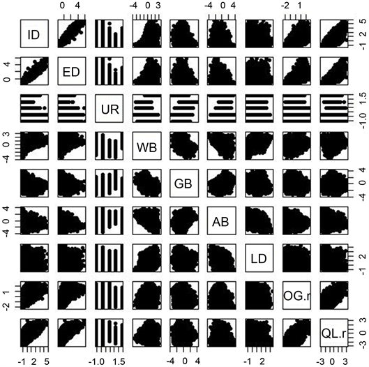
We shall create a Database for predictive variables and then plot the scatter plots for pairs of the predictive variables. The next step is to check the variables if some are correlated. We first plotted the scatter plots for pairs of the predictive variables to see how they are correlated. If two variables are correlated, we can choose one to represent the other, it is unnecessary to include both variables in the model. The Scatter plots are in form of vectors shown on page 13. From the scatter plot, we found that Employment Deprivation is highly correlated with Income Deprivation. As a result of this, we decided not to include Employment Deprivation in the last model.

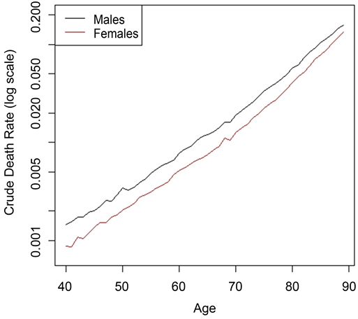
We need to calculate the crude age-specific death rates at the national level for males by summing deaths over all LSOA’s and divide it by the sum of exposures over all LSOA’same. This is followed by plotting some death rates at the national level on log scale and is available on page 14.

In this multiple regression, the next step is to determine which predicted variables contribute significantly to explaining the variability in the standardised mortality ratio. A model that contains all the predicted variables will give the maximum $R^2$ value but our analysis shows that not all variables contribute significantly to explaining the variability in the standardised mortality ratio.

Initialise the vector of deaths and the vector of expected deaths under the NULL model is the next step, to be followed by regressing deaths on the male sex. We have chosen to use male sex since both are similar in all respects. After this, we shall then regress the deaths on the predictive variables.

3.3. Model Selection

The next crucial step is to select the most appropriate model among the model class. This involves selection of a statistical model from the model class that best fit the data by choosing the model that has the smallest AIC value.

When comparing competing models, information criterion-based fit indices are useful. A commonly used measure from the information theoretic tradition is Akaike’s information criterion (AIC). AIC balances the model’s goodness-of-fit to the data and a penalty for model complexity. The general method for using the AIC is to choose the model that has the smallest AIC value. NCSS Statistical Software (2018) expressed that Akaike’s information criterion is equal to the deviance plus twice the number of parameters in the model.

It further expressed that AIC combines a measure of the discrepancy between the fitted values and the data (the deviance) with a measure of the simplicity of the model (twice the number of parameters). It has been shown by NCSS that using AIC to compare competing models with different numbers of parameters amounts to selecting the model with the minimum estimate of the mean squared error of prediction.

In essence, having to remove Employment deprivation because it is highly correlated with income deprivation and Geo Barriers due to its statistical insignificance, our Poisson regression model, with the least AIC, has six predictive variables. The model summary is as follows:

glm(formula = D ~ ID + AB + OG.r + UR + LD + WB, family = poisson, offset = log(Dhat)).

4. Results

We found that income deprivation is the strongest independent predictor of mortality rates in a neighbourhood. Each of the variables is statistically significant at less than 5% except for wider barriers that are statistically significant at 5%.

Besides, from the regression analysis, we found that about 28% of the variation in mortality across LSOAs is explained by income deprivation, occupation group proportions, living deprivation and wider barriers. Income deprivation alone explains about 17% of the variation in mortality rates between LSOAs which is greater than the predictive power of all other variables combined.

The income deprivation index is partly derived from rates of job-seeker’s Allowance which is also included in the derivation of the unemployment deprivation index. The correlation between income deprivation and employment deprivation is very high suggesting unemployment plays a significant role in income deprivation in a neighbourhood.

Our analysis shows that at the age range from 40 to 89 years in males, it is clear that there has been a substantial reduction in mortality rates in all areas regardless of deprivation.

5. Relative Risk

The relative risk is often used when there is a need to compare the possibility of an event occurring between two sections of society. It utilizes the probability of an event occurring in group A compared to event occurring in group B. A relative risk of less than one in A implies that the risk of an event occurring in A is less than the risk of risk occurring in B.

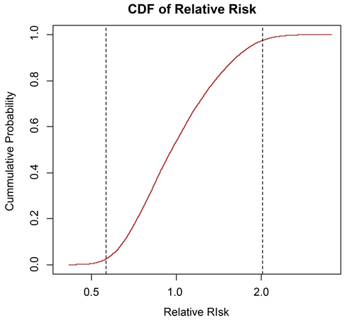
With 2015 deaths data, the Relative Risk was calculated with six coefficients showing that 2.5% and 97.5% quartiles are respectively 0.563755 and 2.016896. This shows that more than 2.5% of the population of the LSOA has 2 times mortality more than the national average mortality. The cdf plot is available on page 14.

The crude death rate on a log scale was shown in a separate sheet showing an increasing mortality rate as the age gets increasing but the mortality in men are higher than women mortality as expected.

6. Conclusion

Our analysis shows that income deprivation, as estimated from state benefits and largely associated with unemployment, is the strongest independent predictor of mortality rates in a LSOA neighbourhood. We equally found out that as the predictive variables are being added to the model, the Poisson Regression model keeps improving better, owing to the fact that the AIC keeps reducing.

Our analysis further revealed that using the log of the standardised mortality ratio (ln(SMR)) as the dependent variable provided a better fit than using the untransformed SMR.

Appendices

Scatter plots of predictive variables

Conflicts of Interest

The authors declare no conflicts of interest regarding the publication of this paper.

References

[1]	Barboutsos, A., de Beer, J., & Janssen, F. (2018). Projecting Delay and Compression of Mortality. Genus, 74, Article No. 17. https://doi.org/10.1186/s41118-018-0039-5
[2]	Bergeron-Boucher, M., Canudas-Romo, V., Pascariu, M., & Lindahl-Jacobsen, R. (2018). Modelling and Forecasting Sex Differences in Mortality: A Sex-Ratio Approach. Genus, 74, Article No. 20. https://doi.org/10.1186/s41118-018-0044-8
[3]	Booth, H., Hyndman, R. J., Tickle, L., & De Jong, P. (2006). Lee-Carter Mortality Forecasting: A Multi-Country Comparison of Variants and Extensions. Demographic Research, 15, 289-310. https://doi.org/10.4054/DemRes.2006.15.9
[4]	Booth, H., Maindonald, J., & Smith, L. (2002). Applying Lee-Carter under Conditions of Variable Mortality Decline. Population Studies, 56, 325-336. https://doi.org/10.1080/00324720215935
[5]	Booth, H., & Tickle, L. (2008). Mortality Modelling and Forecasting: A Review of Methods. Annals of Actuarial Science, 3, 3-43. https://doi.org/10.1017/S1748499500000440
[6]	Bozikas, A., & Pitselis, G. (2019). Credible Regression Approach to Forecasting Mortality for Populations with Limited Data. Risks, 7, 27. https://doi.org/10.3390/risks7010027
[7]	Cairns, A. J., Blake, D., & Dowd, K. (2006). A Two Factor Model for Stochastic Mortality with Parameter Uncertainty: Theory and Calibration. Journal of Risk and Insurance, 73, 687-718. https://doi.org/10.1111/j.1539-6975.2006.00195.x
[8]	Cairns, A. J. G., Blake, D., Dowd, K., Coughlan, G. D., Epstein, D., Ong, A., & Balevich, I. (2009). A Quantitative Comparison of Stochastic Mortality Models Using Data from England and Wales and the United States. North American Actuarial Journal, 13, 1-35. https://doi.org/10.1080/10920277.2009.10597538
[9]	Cerda-Hernandez, J., & Sikov, A. (2018). Lee-Carter Method for Forecasting Mortality for Peruvian Population. https://www.researchgate.net/publication/329210190
[10]	Chambers, J. M., & Hastie, T. J. (1992). Statistical Models in S. London: Chapman & Hall.
[11]	Currie, I. D. (2018). Fitting Models of Mortality with Generalized Linear and Non-Linear Models.
[12]	Diaz, G., & Debón, A. (2018). Mortality Forecasting in Colombia from Abridged Life Tables by Sex. Genus, 74, 15. https://doi.org/10.1186/s41118-018-0038-6
[13]	Eager, C. (2017). Standardize: Tools for Standardizing Variables for Regression in R. https://www.researchgate.net/publication/316789685
[14]	Fazle Rabbi, A. M., & Mazzuco, S. (2018). Mortality and Life Expectancy Forecast for (Comparatively) High Mortality Countries. Genus, 74, Article No. 18. https://doi.org/10.1186/s41118-018-0042-x
[15]	Gelman, A. (2008). Scaling Regression Inputs by Dividing by Two Standard Deviations. Statistics in Medicine, 27, 2865-2873. https://doi.org/10.1002/sim.3107
[16]	Janssen, F. (2018). Advances in Mortality Forecasting: Introduction. Genus, 74, Article No. 21. https://doi.org/10.1186/s41118-018-0045-7
[17]	Lee, R. D., & Carter, L. R. (1992). Modelling and Forecasting US Mortality. Journal of the American Statistical Association, 87, 659-671. https://doi.org/10.1080/01621459.1992.10475265
[18]	Li, H., & O’Hare, C. (2017). Semi-Parametric Extensions of the Cairns-Blake-Dowd Model: A One-Dimensional Kernel Smoothing Approach. Insurance: Mathematics and Economics, 77, 166-176. https://doi.org/10.1016/j.insmatheco.2017.10.001
[19]	Marius, D. P. (2018). Modelling and Forecasting Mortality. PhD Thesis, Odense: University of Southern Denmark.
[20]	NCSS Statistical Software (2018). Poisson Regression. Chapter 325. https://www.ncss.com/
[21]	Renshaw, A. E., & Haberman, S. (2006). A Cohort-Based Extension to the Lee-Carter Model for Mortality Reduction Factors. Insurance: Mathematics and Economics, 38, 556-570. https://doi.org/10.1016/j.insmatheco.2005.12.001
[22]	Shang, H. L., & Haberman, S. (2018). Model Confidence Sets and Forecast Combination: An Application to Age-Specific Mortality. Genus, 74, Article No. 19. https://doi.org/10.1186/s41118-018-0043-9
[23]	Stoeldraijer, L., van Duin, C., van Wissen, L., & Janssen, F. (2013). Impact of Different Mortality Forecasting Methods and Explicit Assumptions on Projected Future Life Expectancy: The Case of the Netherlands. Demographic Research, 29, 323-354. https://doi.org/10.4054/DemRes.2013.29.13
[24]	Stoeldraijer, L., van Duin, C., van Wissen, L., & Janssen, F. (2018). Comparing Strategies for Matching Mortality Forecasts to the Most Recently Observed Data. What Is the Best Trade-Off between Short-Term Accuracy and Long-Term Robustness? Genus, 74, Article No. 16. https://doi.org/10.1186/s41118-018-0041-y
[25]	Villegas, A. M., Millossovich, P., & Kaishev, V. K. (2018). StMoMo: Stochastic Mortality Modeling in R. Journal of Statistical Software, 84, 1-38. https://doi.org/10.18637/jss.v084.i03
[26]	Waldron, H. (2005). Literature Review of Long-Term Mortality Projections. Social Security Bulletin, 66, 16-30.
[27]	Wilson, T. (2018). Evaluation of Simple Methods for Regional Mortality Forecasts. Genus, 74, 1-22. https://doi.org/10.1186/s41118-018-0040-z