The Bare and Dressed Masses of Quarks in Pions via the of Quarks’ Geometric Model

Giovanni Guido

Department of Physics and Mathematics, High Scholl “C. Cavalleri” Parabiago, Milano, Italy.

DOI: 10.4236/jhepgc.2019.54065                

Abstract

In previous articles (Guido) we demonstrated that Quarks (u, d) are represented by golden geometric structures of coupled quantum oscillators. In this article we show the geometric structure of the pion triplet and, in particular, via the structure equation of neutral pion, we identify its decays and we solve the spin question in hadrons thanks also to introduction of algebraic operations [?, ⊕] on geometric structure. Moreover by means of the golden ratio between (u, d), we determine the values of bare masses of quarks (3.51 MeV for u-quark and 5.67 MeV for d-quark) and those ones bounded in a pion (53.31 MeV for u-quark and 85.26 MeV for d-quark). Finally, using algebraic operations [?, ⊕] we point out a new way to represent the processes of pions’ decay.

Keywords

Quark, Structure Equation, Geometric Structure, Golden Number, Massive Coupling, Interpenetration, IQuO, Semi-Quantum, Pion, Photon

1. Introduction

A problematic aspect in Hadrons (see literature [1] [2] ) is that one only a small fraction of a hadron mass seems to be associated to the mass of the elementary quarks (see the idea of bare mass in a free quark). In fact, in phenomenology of the hadronic interactions, the masses of a quark (u, u, d) forming the proton (see literature) seem around 10 MeV [3] [4] : in this way a quark would represent only ~1% of the proton mass. This is a really critical issue regarding the mass of the hadrons, seen as quarks’ structures. This aspect could be connected to the hypothesis [2] that an isolated quark cannot exist by itself, see the process of Hadronization: in this framework the idea of a free (or bare) mass in quarks doesn’t seem to have any sense. Actually, the possibility of speaking about free quarks seems more strong when one observes the productions of hadronic jets in collisions of high energy at CERN. Nevertheless, nowadays the mass question of quarks doesn’t seem to be resolved: any quantitative statement about the value of a quark mass must make reference to the particular phenomenon in which the quark is observed. The actual literature states that quarks (u and d) have the following experimental range of values of free masses [4] :

$m_u=\text{range}\left[\text{1}.\text{7}\text{-}\text{3}.\text{3}\right]\text{MeV}$

$m_d=\text{range}\left[\text{4}.\text{1}\text{-}\text{5}.\text{8}\right]\text{MeV}$

Unlike leptons, these values are always referred to quarks seen confined inside hadrons and not observed directly as physical particles. So, we would still admit that quarks’ masses can be determined indirectly by their influence on hadronic properties.

Nowadays, one of the answers to the mystery of mass origin in hadrons is the fact that the mass remaining fraction is due to the force (gluons) binding the quarks within hadrons, i.e. Quantum Chromo Dynamics (QCD). This way one thinks that the values of the quark masses, obtained [5] directly in lattice simulations, are “bare” masses of quarks, corresponding to a particular discretization of QCD. In these simulations some values of experimental masses [5] are used as input (see the pion mass) to improve the mass and coupling parameters in the interactions in order to calculate the masses of hadrons. The pion so playing a fundamental rule for calculating the masse of mesons. Instead we’ll use the masses of pion triplet for calculating the masses of their component quarks (u, d) both bonded inside the pion that the bare ones.

Nevertheless, all of this will be possible only if we affirm [6] [7] the quarks having a well-defined geometric structure; this idea of geometric structure can be achieved if we assume [6] a quark is made by a not separable set of coupled quantum oscillators. We will refer to this as the Geometric Model of quarks (GM) where these cannot be punctual objects (see the Quantum Relativistic Theory of fields), but geometric forms of coupled oscillators. Thanks to the quarks geometric hypothesis, it is possible to explain fundamental issues such as the origin of the hadrons mass and quarks. As soon as one defines the particular geometric form then it is possible formulating a structure equation with which can calculate the masses of quarks and mesons. In particular, we determine in this paper the structure equation of pion neutral.

Nevertheless, for obtain the masses (and, in a following study, the nucleons ones as well) we need to revise the mass conception in physics and introduce a new idea of mass calculation (Ä-operation), which takes into account both interactions between quarks and a possible interpenetration of the quarks (this is an aspect purely quantum-mechanical like to superposition of waves). The latter may exist only if we admit different structures of coupled quantum oscillators (or quarks) in overlapping without exchanging energy. The global mass of hadron must therefore take into account all the possible configurations of quark components, both the ones with interpenetration and the ones with interactions.

The hypothesis of quark geometrical structure introduces a new paradigm (see GM) in the phenomenology of hadronic interactions, suggesting the quarks have an internal geometrical structure. Thanks to a few basic hypotheses, the new paradigm allows instead to describe the hadronic phenomenology in a more structured and simple way. A first evidence will be given by calculating the spectrum of light mesons with mass values very close (if not even equal) to the experimental ones. In this paper we formulate the structure equation of pion and its decays and we solve the spin question in hadrons. The interpenetration of quarks is connected to an intrinsic internal movement which well explains the total spin of pion as sum of more components of the spin connect to different parts of quark in movement.

Moreover thanks to golden form of quarks inside pion, we calculate the mass values of quarks (u, d) inside to pion, and, through structure equation of neutral pion, also those ones of bare masses.

Finally, using algebraic operations [Ä, Å] we point out a new way where to represent the processes of pions’ decay.

2. The Quarks as Coupling Quantum Oscillators

2.1. The Hypothesis of Structure

In ref. [6] [7] we have recalled the wave behaviour of particles which could induce us to admit that something oscillates within a particle. Then it needs to talk about an oscillation (a clock) inside the particle with a proper frequency of pulsation (ω₀). Moreover, talking about the Compton wavelength (Δ_c) or spin in massive particle, then we can speak of space inside them. All this could lead us to affirm the Space-Time (ST) being intrinsic to massive particles. Moreover, talking about Space-Time (ST) inside a massive particle, it’s exactly the same as talking about an internal structure of particle. If we want to talk about internal oscillations to particle, seen as structures, but at the same time to be coherent with the relativity and Quantum Mechanics, then only one assertion is possible: particles could be geometric structures of coupled quantum oscillators. Recall the quantum theory of fields where particles are sets of coupled quantum oscillators, then it’s intuitive to give a structure of coupled oscillators to massive elementary particles: this is the idea of hypothesis of structure [6]. A note should be made here: the coupled quantum oscillators constitute a unique physics object, defined particle, to which a wave function Ψ(x, y, z, t) in a point of ST is associated. These aspects already have been treated in previous papers [6] [7] where we have established that quarks are structures of coupled oscillators with a geometric form. In this way we speak of a Geometric Model (GM) of the quarks and in general also of any particle.

To assign a geometric structure to coupled oscillators is equivalent to assign a proper frequency (ω₀) to them, or an oscillation period (τ) coinciding, in relativity, with the proper time.

The proper characteristic of a massive particle, associated with the proper time (τ) of an object, coincides with the proper mass (m₀). To speak of the mass or mass energy of a particle, it is the same as speaking the time of the clock that is inside them [ω₀ ó τ ó m₀]. Then, based on QM [8] :

$\left\{\begin{array}{c}{E}_0=m{c}^2\\ E_0=\hslash {\omega }_0\end{array}\right\}\Rightarrow \left\{m=\frac{\hslash {\omega }_0}{c^2}\right\}$ (1)

If the frequency (ω₀) origins the proper time (τ) of a massive particle [τ = h/mc²], then for symmetry, exists a wavelength (Δ) that origins the “proper space” of the particle. Following De Broglie, it’s:

$\{\begin{array}{l}{p}_0=mc\\ p_0=\hslash \frac{2\pi }{{\lambda }_0}\end{array}\Rightarrow {ƛ}_0=\frac{\hslash }{mc}\equiv {ƛ}_c$ (2)

The equation [(ω₀Δ) = (Δ/τ) = c] is the dispersion relationship in the Space-Time 4-dim of a reference frame “at rest” (S˚) where the wave is “a rest” or where an observer notes only a stationary oscillation and do not observes the “progression” of the wave.

Combining the equation of the relativistic energy of massive particle in movement (velocity (v)) in a reference frame (S) with the equations of Einstein (1) and De Broglie (2) we have:

$\left\{E^2=m^2{c}^4+p^2{c}^2\iff {\omega }^2={\omega }_0^2+k^2{c}^2\right\}$ (3)

This is the dispersion relationship of waves propagating in (S), as described by the Klein-Gordon equation:

$\left\{\frac{{\partial }^2\Psi \left(x,t\right)}{\partial t^2}=c^2\frac{{\partial }^2\Psi \left(x,t\right)}{\partial x^2}-{\omega }_0^2\Psi \left(x,t\right)\right\}$ (4)

As is well known, this equation describes both the oscillations in a set of coupled pendulums through springs [9] and a scalar fields associated to massive particles with zero spin (see pion):

$\left\{\frac{{\partial }^2\Psi \left(x,t\right)}{\partial x^2}-\frac{{\partial }^2\Psi \left(x,t\right)}{c^2\partial t^2}={\left(\frac{mc}{\hslash }\right)}^2\Psi \left(x,t\right)\right\}\iff \left\{{\nabla }^2\Psi \left(x,t\right)={\left(\frac{mc}{\hslash }\right)}^2\Psi \left(x,t\right)\right\}$ (5)

We conjectured [6] that mass is a physical expression of the proper frequency (ω₀) related to a particular elastic coupling, which is in addition to the one already existing between the oscillators of the massless scalar field (X). This “additional coupling” which produces the mass in a scalar field (X), has been referred to as a “massive coupling”. Then, we conjectured that the massive particle-field (X) is created by a “transversal coupling” (T₀) between the chains of oscillators of the scalar base field (X). This can be depicted figuratively as shown in Figure 1.

When we observe only the oscillation with frequency (ω₀) in all points (x) then we are at rest with the massive particle (m ó ω₀ ó T₀) and this aspect is coincident to the that in which the springs do not are involved. Instead when the springs are involved the wave becomes progressive with frequency (ω) wave length (λ) and represent a massive particle with velocity (v) (see Equation (3)).

Figure 1. Massive field as lattice of “pendulums” with springs.

2.2. The “Golden” Particles

Let us note the relationship between the Compton’s wavelength of the proton and that of Planck’s particle [6] [7]. If we indicate with n_(pl,p) the experimental numerical ratio between the Compton’s wave length (Δ_pl) and (Δ_p), experimentally it’s:

$\left(n_{\left(pl,p\right)}\right)=\left(\frac{{ƛ}_p}{{ƛ}_{pl}}\right)=\left(\frac{m_{pl}}{m_P}\right)=\left[\frac{\text{2}\text{.176450}\times {10}^{-8}}{\text{1}\text{.672623}\times {10}^{-27}}\right]=\text{1}\text{.301}\times {10}^{19}$ (6)

the power (10)^(p) can be a representative scale factor (s).

Recall: ${\varphi }^2={\left(1.618\right)}^2={\left(2.618\right)}^2$

Where ( $\varphi$ ) is the “aureus” (golden) number. Note $\left[n_{\left(pl,p\right)}/{10}^{19}\right]~\left[{\varphi }^2/2\right]$ and $\left[2n_{\left(pl,p\right)}={\varphi }^{2}s\right]$. Between Compton’s wave length (Δ_pl) and (Δ_p) there is so a golden relation, at less than a s-scale factor (10)^p. Recall the golden segments (see Figure 2).

By property of the golden segments it’s:

$\{\begin{array}{l}{ƛ}_{\beta }=\left(\frac{{ƛ}_{\gamma }}{\varphi }\right)\\ {ƛ}_{\gamma }={\varphi }^2{ƛ}_{\alpha }\end{array}$ (7)

These relations there are in a pentagon between the side and apothem. As is well known in literature, the protons are composed of three quarks: three centres of diffusion positioned in a triangular form in diffusion experiments with “bullet” electrons. These centres indicate (Figure 3) the proton having an internal geometric structure.

By the Hypothesis of Structure, we could conjecture a proton having a “pentagonal” geometric structure where the three component quarks are coincident with three constituent triangles, see Figure 3.

The scale factor (10)^p of proton relative to Plank’s particle can be due to expansion of universe which maintains invariant the relation between physical quantities.

Then we could state proton like golden particle; by Figure 3, the three aureus triangles (u, u, d) may be three “coupled” quarks. The Structure Hypothesis induces to put in the vertices (A, B, D) three quantum oscillators with which a photon couples in the electromagnetic interactions: in fact, [10] [11] in diffusion

Figure 2. “Aureus” segments.

Figure 3. Geometric structure at quark of the proton.

processes (e + p), investigating the internal structure of the proton, three diffuser center are highlighted in triangular form. Still considering diffusion processes, we have conjectured (see Figure 3) that the diagonals (AD) or (BD) are proportional to Compton wavelength assigned to the proton. In pentagonal structure, it’s evident that the diagonals [(AD), (BD)] are in a golden ratio with the base AB:

$\left(\varphi =1.618\right)\to \left[\left(\text{AD}/\text{AB}\right)=\varphi \right]$.

This implies also quarks (u, d) are aureus triangles. We have (see Equation (7)):

$\left\{\begin{array}{c}{ƛ}_u={ƛ}_{\gamma }\\ {ƛ}_d={ƛ}_{\beta }\end{array}\right\}$

A geometric property of the golden triangles (u or d) is that one each triangle is composed in its turn of two golden triangles, see Figure 4 and ref. [6].

Because the supporting diagonals in the proton are essential for its structure, it’s conjectured that the side (AD)_p (in Figure 3) of quark (u) can be proportional to Compton wavelength of proton (Δ_p = h/m_pc), thus: [Δ_p = k_pΔ_u].

Where (Δ_u) is the Compton wavelength of “free” quark, while (k_p) is a coefficient of “elastic adaptation” when (u, d) quarks reciprocally bind for origin the proton. Just k_p can be in relation with binding gluons of the (u, d) quarks into proton; we’ll point out [V(r)_QCD ó k_p], where V(r) is gluonic potential in QCD theory [12] [13]; so in this theory the potential V(r) is replaced by elastic tension k. Moreover, the diagonal (AD) in u-quark (Figure 3) can represent the transverse coupling that supports the structure of the coupled quantum oscillators composing it; also the side (AB) in (d-quark) can represent the transverse coupling that supporting the structure of quantum oscillators. From Compton wavelength, the ratio between the masses (both bare and bounded) of the two fundamental quarks will be:

Figure 4. Golden triangles (u₁, d₁) into golden triangle (u, d).

$\left[\left({ƛ}_u/{ƛ}_d\right)=\left(m_d/m_u\right)=\varphi \approx 1.618\right]$ with ( $m_d>m_u$ ).

These internal oscillators have been indicated [6] [7] with acronym IQuO (Intrinsic Quantum Oscillator). Their geometric form is depicted by three spheres (IQuO-Vertex) being placed at the vertices of a golden triangle and connected by springs (Joining IQuO). Because the three quantum oscillators constitute a unique physical object, i.e. a unique quark, they cannot be detected separately, as shown in Figure 5.

Straight away we notice that this structure is realizable only through “particular” quantum oscillators. This “particularity” is underlined into necessity that the vertex—oscillators and junction oscillators must have a structure of “hooks”: this induces us to talk about a “sub-structure” into quantum oscillator which is highlighted only into quantum oscillator coupled to other oscillators. It’s evident that the sides of this structure are made with “additional coupling” between quantum oscillators: there is so one only frequency of oscillation for whole structure (ω₀ ó m₀). As we have already note in previous articles [6] [7], indication of a “composite structure” in quantum oscillator can be derived from its wave function. In fact, the quantum oscillator (with n the quantum number and n = 1) shows a wave function (Ψ) with a pair of peaks in the probability of detecting the energy quanta of the oscillation, see Figure 6: we can describe therefore the quantum oscillator with two sub-units of oscillation or “sub-oscillators”. Into [7] quantum oscillator with (n = 2) there are three peaks in wave function (Ψ) which denote three sub-oscillators, Figure 6.

Not only but more components in an oscillator encourages us to believe that the energy of the “quanta” should be distributed between these oscillating components. The presence of more components in an oscillator causes the splitting of its quanta of energy into two, and more, sub-oscillators: this introduces the idea of half-quanta (“semi-quanta”) or individually half-quantum (“semi-quantum”).

Recall in quantum oscillator the energy levels: $\left[{\epsilon }_n=\left(n+\frac{1}{2}\right)h\nu \right]$. For (n = 1) is $\left[{\epsilon }_1=\left(1+\frac{1}{2}\right)h\nu \right]$ ; with two sub-oscillators the probability function P₁(x) of energy distribution, Figure 7, will be:

Note [ε₀ = (1/2)hω)] indicates a semi-quantum, while [ε = (1)hω) = 2(1/2)hω] represents one quantum composed by two “entangled” semi-quanta. We so can think that the “IQuO” inside quarks are quantum oscillators at “semi-quanta”. A quantum oscillator with a sub-structure constituted by sub-unit of oscillation, or

Figure 5. Quark sub-structure.

Figure 6. Probability function of quantum oscillator.

Figure 7. Probability function in quantum oscillator in energy eigenstate with (n = 1).

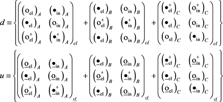
“sub-oscillators”, and “semi-quanta” is an oscillator of type “IQuO” [7]. Its mathematic structure is that one of quantum oscillator with annihilation operator (a) and creation (a⁺):

$\begin{array}{l}\left[\Psi \left(t\right)\right]\equiv \left(\begin{array}{c}{\hat{a}}_{r^{\prime }}^{+}\left(t\right)\\ {\hat{a}}_{r^{\prime }}\left(t\right)\end{array}\right)=\{\begin{array}{l}{\hat{a}}_{r^{\prime }}^{+}\left(t\right)={\left({\widehat{•}}^{+}\right)}_{\text{el}}\left[\exp \left(i{r}^{\prime }\omega t\right)\right]+{\left({\hat{\mathrm{o}}}^{\text{+}}\right)}_{\text{in}}\left[\exp \left(i\left(r^{\prime }\omega t-\pi /2\right)\right)\right]\\ {\hat{a}}_{r^{\prime }}\left(t\right)={\left(\hat{\mathrm{o}}\right)}_{\text{el}}\left[\exp \left(-i{r}^{\prime }\omega t\right)\right]+{\left(\widehat{•}\right)}_{\text{in}}\left[\exp \left(-i\left(r^{\prime }\omega t-\pi /2\right)\right)\right]\end{array}\\ \text{with}\stackrel{\to }{\Psi }\left(t\right)\equiv \left[{\stackrel{\to }{a}}^{+}\left(t\right)+\stackrel{\to }{a}\left(t\right)\right]=\left[\left(a_{\text{el}}^{+}\left(t\right)+a_{\text{in}}^{+}\left(t\right)\right)+\left(a_{\text{el}}\left(t\right)+a_{\text{in}}\left(t\right)\right)\right]\end{array}$

where [(·), (o)] are the components of [a, a⁺] and operators of full semi-quantum (·) and empty semi-quantum (o). To treat the particles as IQuO structures can explain the origin of some fundamental physics greatness as the electric charge, spin, isospin and color charge [7]. So, the IQuO idea constitutes a new paradigm in physics which allow us of describes with depth the physical phenomenon of particles and to open new descriptive scenarios of interactions between particles. The overlapping of a sub-oscillator of IQuO (I₁) with another of IQuO (I₂) makes a coupling between two IQuO (I₁) and (I₂): [(I₁) Ç (I₂)]. In ref. [7] we have showed as one builds the structure of Figure 5, realizing the u-quark and d-quark. We said that all sides are made by “double” sub-oscillators in overlapping and each of these is a gluons.

The representative matrix [7] of a vertex IQuO_(n=2*) (with n = 2* because it is composed by 3 sub-oscillators with 3 full semi-quanta (·)) will be represented by a column matrix with three elements:

${\left(\left(\Psi \right)\right)}_{cl}={}_3\left(\begin{array}{c}\left({\hat{\mathrm{o}}}_{\text{el}}{e}^{-i\rho }+{\widehat{•}}_{\text{in}}{e}^{-i\rho °}\right)\\ {\left({\widehat{•}}_{\text{el}}{e}^{-i\alpha }+{\hat{\mathrm{o}}}_{\text{in}}{e}^{-i\alpha °}\right)}_c\\ \left({\hat{\mathrm{o}}}_{\text{el}}^{+}{e}^{-i\sigma }+{\widehat{•}}_{\text{in}}^{+}{e}^{-i\sigma °}\right)\end{array}\right)$

where [(α° = α + π/2), (ρ° = ρ − π/2), (σ°= σ ± π/2)].

The index (cl) point out the clockwise associated to d-quark, which is represented (omitting the junctions’ IQuO) by an overlapping of three IQO-V [(I_A(+) I_B(+) I_C)]:

$\left\{{\left(\begin{array}{c}\begin{array}{cc}{\left({\text{o}}_{\text{el}}\right)}_A& {\left({•}_{\text{in}}\right)}_A\end{array}\\ \begin{array}{cc}{\left({•}_{\text{el}}\right)}_A& {\left({\text{o}}_{\text{in}}\right)}_A\end{array}\\ \begin{array}{cc}{\left({\text{o}}_{\text{el}}^{+}\right)}_A& {\left({•}_{\text{in}}^{+}\right)}_A\end{array}\end{array}\right)}_{cl}+{\left(\begin{array}{c}\begin{array}{cc}{\left({•}_{\text{el}}\right)}_B& {\left({\text{o}}_{\text{in}}\right)}_B\end{array}\\ \begin{array}{cc}{\left({\text{o}}_{\text{el}}^{+}\right)}_B& {\left({•}_{\text{in}}^{+}\right)}_B\end{array}\\ \begin{array}{cc}{\left({•}_{\text{el}}\right)}_B& {\left({\text{o}}_{\text{in}}\right)}_B\end{array}\end{array}\right)}_{cl}+{\left(\begin{array}{c}\begin{array}{cc}{\left({•}_{\text{el}}^{+}\right)}_C& {\left({\text{o}}_{\text{in}}^{+}\right)}_C\end{array}\\ \begin{array}{cc}{\left({•}_{\text{el}}\right)}_C& {\left({\text{o}}_{\text{in}}\right)}_C\end{array}\\ \begin{array}{cc}{\left({\text{o}}_{\text{el}}\right)}_C& {\left({•}_{\text{in}}\right)}_C\end{array}\end{array}\right)}_{cl}\right\}$

(omitting the phases)

By matrices we can make the various coupling between quarks and so to build the structure representatives of hadrons.

Finally, we do not must thinking to a rigid structure of quarks: different orientations in space are possible (see Figure 3) of triangles ADE and BCD around the diagonals AD and BD, as even the triangle ABD around AD or BD. This last aspect can origin the spin of quarks inside a proton. Recall the coupling quantum oscillators of particle are an “oneness”, therefore the spin is always described by properties of wave function in presence of different orientations of observations (see the Pauli’s matrices).

Note: talking about a geometric structure of coupling oscillators in quarks, implicitly it’s giving mass values not zero to them. Therefore, this quark model describes only “massive quarks”. This will be more evident in next section.

3. The Structure of Pions

3.1. The Structure of Charged π^±

Mesons are hadrons composed of quark-antiquark pairs and the most elementary is the pion. Figure 3 suggests that mesons may be represented by a geometric structure realized by coupling between the golden quarks u and d (see also Figure 4 and [6] ).

A first attempt of structure equation is: [(π⁺) = (u Å d), (π⁻) = (u Å d)].

The sign (Å) point out the dynamics coupling between quarks; it could involve both gluonic coupling and electromagnetic: [Å = Å_g + Å_em].

Then, we have the configuration illustrated in Figure 8.

Figure 8. Geometric form of pion.

Where u is the u antiquark. The double circles indicate the coupling between vertices-oscillators (B ó B’, C ó C’).

The coupling between the u quark and d quark forms so a quadrangular structure (ABDC). The bond (see gluons) between two free quarks (u ó d) increases the elastic tension between IQuO components of quarks [(k_u, k_d) → (k_u, k_d)] which in turn increases the “free” frequencies [(ω_u, ω_d) → (ω_u, ω_d)] or mass [(m_u, m_d)_free → (m_u, m_d)], see Equation (1); thus the Compton wavelength decreases ( ${\underset{\_}{ƛ}}_u$ < ${ƛ}_u$ ), ( ${\underset{\_}{ƛ}}_d$ < ${ƛ}_d$ )], shrinking the u and d quarks (see second drawing in Figure 8). Two quarks (u, d) can attach only along the side AC óA’C’ because in golden triangles (u, d) these sides are equal. Once it has finished the phase of attachment, the π-structure is a similar system to two coupled oscillators (u ó d) which oscillate with only one frequency (ω_π) and period (τ_π), to which we associate (Δ_π, m_π). Each quark (u, d) contributes to total mass (m_π) with its mass value (m_u, m_d), maintaining the golden ratio $\left[\left({\underset{\_}{m}}_d/{\underset{\_}{m}}_u\right)=\varphi \right]$. Speaking of elastic tensions in bound quarks we can admit that in the (k_i) are contained the mass defects (recall that k replaces the potential V(r)), so that we have [m_π = m_u + m_d].

The representative quantum of (u-quark)_π oscillates (in the Space-Time (ST)) with proper time ${\left[{\underset{\_}{\sout{\tau }}}_u=\left({\underset{\_}{ƛ}}_u/c\right)\right]}_{\pi }$ and that one of (d-quark)_π with ${\left[{\underset{\_}{\sout{\tau }}}_d=\left({\underset{\_}{ƛ}}_d/c\right)\right]}_{\pi }$, while in bound system (π) the representative quantum oscillates (in ST) with proper frequency (ω_π), with elastic constant (k_π), wave length ${ƛ}_{\pi }$ and proper time ${\left[{\underset{\_}{\sout{\tau }}}_{\pi }=\left({\underset{\_}{ƛ}}_{\pi }/c\right)\right]}_{\pi }$.

Note, instead, the representative quantum of (u-quark)_π covers the route (BDC ó l_u) in time [Δτ_u = (l_u/v_u)]_π and that one (ABC ó l_d) of (d-quark)_π in [Δτ_d = (l_d/v_u)]_π, in bound system (π) the representative quantum covers the route (ABDC ó l_π) in time [Δτ_π = (l_π/v_π)]_π.

In this case we’ll have that the periods of route in u-quark and in d-quark must be coincident with that of π-structure: [Δτ_u = Δτ_d = Δτ_π]. This indicates that the velocities of propagation of quanta in the structures (u, d, π) are different because are different the elastic tensions of respective sides; recall (see Figure 1) that the propagation of a linear wave impulse is [v²= (T/μ)] with (T ó k) and (μ) is mass density of the chain of coupled oscillators. It follows: (k_u < k_d < k_π) ó (v_u < v_d < v_π).

Where [k_u ó (BDC) óω_u], [k_d ó (ABC) óω_d], [k_π ó (ABDC) óω_π].

As it occurs in Hidrogen atom, where the oscillation period (τ_H) along an orbital is joined to rotation period Δτ_H, so it needs happen in pion: [(τ_π) ó Δτ_π ó (τ_π)].

The experimental mass of pion (m_π) has frequency (ω_π) and period (τ_π); we must point out that: Δτ_π = (τ_π).

By π-structure we point out Δ_π = Δ_u = k_uΔ_u, where Δ_u is the Compton wavelength of the free u quark (m_u is bare mass, k_u internal elasticity of free quark); the Δ_π is the Compton wavelength (side BC) of quadrangular structure (ABDC)_π and is coincident to Δ_u, the Compton wavelength of the u quark bounded inside to pion. Therefore Δ_π > Δ_π, where Δ_π = h/m_πc, indicating that the junction IQuO of side CD can be composed of more quantum oscillators [6] : one of these has linear dimension equal to the Compton wavelength of pion π (see the second configuration of Figure 8).

To the frequency ω_π we associate k_π elastic coefficient, which is related to the gluonic potential V(r) of the QCD and thus in turn is related to coupling (Å), where [Å = (Å_g + Å_em)]. Therefore, even along sides, there are gluons (see the Joining-IQuO of Figure 5) connecting the vertex oscillators. This aspect is consistent with QCD [13].

In the pion, different configurations are related to the X-junction axis, Figure 8. The possible configurations are depicted in Figure 9.

Where I_A, I_B, I_C, I_D, are vertex IQuO, I_AB, I_BC, I_CA, I_BD, and I_DC are junction IQuO. In configuration 1, I_D is an IQuO vertex non-coupled with IQuO of the side AC. The I_D IQuO is free. To tie the two quarks (u, d), it is necessary to add a junction IQuO between the respective bases’ oscillators. We suspect that the IQuO oscillators of the junction between the sides (BC)_d, and (B’C’)_u could be gluons (see Figure 8, or see [7] for an in-depth explanation). The possibility of more relative orientations between two quarks implies a reciprocal rotation of two quarks (u and d) around the X-axis (as orbital motions). Thus, these configurations, or orientations, can induce us to think of the spin of a pion. If we assign the aspect of being a fermion to all structures, then the oscillation propagating along sides is described by a spin wave function. We call this the intrinsic spin of quarks (s_q), while we associate an orbital spin (s_l) to rotations of u-quark (or d-quark) around the X-axis (see the experimental observations about proton spin). The hypothesis of structure does not conflict with experiments of CERN (COMPASS), SLAC, and DESY (HERMES), where the spin of the proton is the sum of intrinsic spins (s_q) of quarks with their orbital motions (s_l); note in rotations around X-axis are involved also binding gluons therefore we add theirs

Figure 9. Pion configurations.

gluonic orbital motion (s_g), as in spin of proton. This model is so consistent with experimental observations [14] [15]. In this way also in pion the total spin is the sum of spin components:

$\left[s_{\pi }=s_q+s_l+s_g\right]$

The possibility of reciprocal rotations of two quarks (u and d) around the X-axis (as orbital motions) induces us to see the quarks as free, and this last word leads us to the behaviour of Asymptotic Freedom of quarks. There are, in fact, no gluons between the vertices (I_A and I_D).

In addition, we may think that the X-axis in Figure 9 is also an axis of pion propagation when this last collapses into an eigenstate of the moment (p_x) along the X-axis. In this way, the X-axis becomes a chain of quantum oscillator pairs (I_B-I_C)_i, of the fermion type, with junction IQuO (I_BC)_i of global length (Δ_π): [(I_B-I_BC-I_C)_i…(I_B-I_BC-I_C)_(i+n)…(I_B-I_BC-I_C)_k…].

As Figure 9 illustrates, each triplet (I_B-I_BC-I_C)_i is part of a quadrangular structure (ABDC) of coupled IQuO. Note only quanta of the pion field propagate along this chain with scalar wave function Ψ(x, t) (see the Heisenberg relation and Equation (5)).

3.2. The Masses of Quarks (u and d) into a Charged Pion of Charged π^±

Now, we calculate the mass of quarks inside the pion: (u_π, d_π) are the bound quarks. We consider $\left(m_d/m_u\right)=\varphi \approx 1.618$ (see Equation (7)). Then, we conjecture that the golden ratio is also present in bound quarks in a pion:

$\{\begin{array}{l}\underset{\_}{m}\left(u_{\pi }\right)+\underset{\_}{m}\left(d_{\pi }\right)=m_{\pi }^{\pm }\\ \underset{\_}{m}\left(d_{\pi }\right)/\underset{\_}{m}\left(u_{\pi }\right)=\varphi \end{array}$ (8)

This equation has solutions

$\{\begin{array}{l}\underset{\_}{m}\left(u_{\pi }\right)=\frac{m_{\pi }^{\pm }}{\left(1+\varphi \right)}=\frac{m_{\pi }^{\pm }}{2.618}=\left(\text{53}\text{.31}\right)\text{MeV}\\ \underset{\_}{m}\left(d_{\pi }\right)=m\left(u_{\pi }\right)\varphi =\left(\text{86}\text{.26}\right)\text{MeV}\end{array}$ (9)

where m(π^±) ≈ (139.57) MeV; see ref. [16]. In Equation (8), we transform the masses in Compton lengths

$\begin{array}{l}\left\{\underset{\_}{m}\left(u_{\pi }\right)+\underset{\_}{m}\left(d_{\pi }\right)=m_{\pi }^{\pm }\right\}\\ \Rightarrow \left\{\left(\frac{\hslash }{ƛ\left(u_{\pi }\right)c}\right)+\left(\frac{\hslash }{ƛ\left(d_{\pi }\right)c}\right)=\left(\frac{\hslash }{{ƛ}_{\pi }c}\right)\right\}\\ \Rightarrow \left\{\left(\frac{\hslash }{{\underset{\_}{ƛ}}_{u}c}\right)+\left(\frac{\hslash }{{\underset{\_}{ƛ}}_{d}c}\right)=\left(\frac{\hslash }{{ƛ}_{\pi }c}\right)\right\}\\ \Rightarrow \left\{\frac{{\underset{\_}{ƛ}}_d+{\underset{\_}{ƛ}}_u}{{\underset{\_}{ƛ}}_u{\underset{\_}{ƛ}}_d}=\frac{1}{{ƛ}_{\pi }}\right\}\Rightarrow \left\{{ƛ}_{\pi }=\left(\frac{{\underset{\_}{ƛ}}_u{\underset{\_}{ƛ}}_d}{{\underset{\_}{ƛ}}_d+{\underset{\_}{ƛ}}_u}\right)={\underset{\_}{ƛ}}_u\left(\frac{1}{1+\varphi }\right)\right\}\\ \Rightarrow \left\{{ƛ}_{\pi }={\underset{\_}{ƛ}}_u/{\varphi }^2\right\}\Rightarrow \left\{{ƛ}_{\pi }={\underset{\_}{ƛ}}_{\pi }/{\varphi }^2\right\}\end{array}$

where Δ_π = Δ_u and Δ_π < Δ_u = Δ_π. We indicate the side BC (Figure 8) as the Compton wavelength of the adapted pion (Δ_π) to a quadrangular structure (ABDC): BC = Δ_π.

k_π is the parameter of calibration that adapts the pion to the bound u quark, which be part of it: $k_{\pi }=\left({\underset{\_}{ƛ}}_{\pi }/{ƛ}_{\pi }\right)=\left({\varphi }^2\right)$. We assign the mass values of Equation (9) to the physical system composed by quarks and gluons that form the pion; the u_π and d_π quarks with their gluons are called dressed quarks. The u_π and d_π quarks are always detected by any observer like a unique quantum system with non-separated components.

3.3. The Interpenetration of Quarks

As noted, different relative orientations between u quarks and d quarks imply a relative rotation (spin) of one quark around the other quark, suggesting a mutual crossing of the quarks (see the overlapping of [I_DC]_u and [I_AC]_d in Figure 9). This crossing can have the meaning of a reciprocal interpenetration between quarks. During this mutual crossing, no energy is exchanged between quarks in those parts that interpenetrate (in the diagonal BC of Figure 8, instead there is an exchange of binding quanta). An analogous phenomenon occurs in waves that cross. Thus, the interpenetration and spin are reciprocally correlated [Interpenetration ó Spin]: this correlation is an aspect purely quantum, so as both the interpenetration and spin. The quantum aspect derives from associate more configurations (eigenstates) of relative orientations between two quarks, simultaneously (no local state). The interpenetration leads us to review the concept of mass. In Newton’s dynamics, mass is the resistance of an object (or inertia) to external actions on it. With this definition, the object’s mass can be physically defined only in interacting objects because, in Newtonian physics, the mass, force (or interaction), and acceleration are inseparable. Also in relativistic theory the mass is measured if the object interacts with other objects, but the mass idea is subsequently widened because involves the energy: mass energy or at rest energy. The phenomenon of pair annihilation can be accepted only if the mass is an energy form. The mass energy is directly connected to one of transversal additional coupling of the field oscillators in particles. This coupling involves additional quanta of field oscillators, thus expressing an additional energy form of particle (massive energy). The macroscopic aspect of massive energy in a particle object (e.g., a ball) is the mass (or inertia) because, to accelerate a more massive object, the agent field (particle) must interact with greater energy (exchanging more quanta). Two bound massive particles (e.g., two bound atoms) exchange greater energy with an external agent and therefore more strongly resist to external action, also considering the defect mass (see deuton). The mass in interactions is thus an additive property, once added the mass defect. If instead, now we consider particles with a geometric structure of coupled oscillators, then their mass is connected both to massive coupling between oscillators but also to their interpenetrations: the additive property no longer can be applied to the total mass. Precisely, the total mass of two or more particles (quarks) must include all the possible configurations of component masses, both interacting and interpenetrating: this is a quantum aspect and relativistic. Therefore, in a system composed of two bound particles (i.e., the quarks of charged pion), the mass of the composed particle must consider apart from the individual masses also dynamics configurations (see binding energy) and possible configurations of interpenetrations between two particles. All this is in line with the relativistic meaning of mass, seen like massive energy. Moreover, note that the interpenetration between particles imply an intrinsic movement. Then, a quantum and relativistic coupling of interpenetration must admit the possibility that this internal movement of components has a kinetic energy form, called by us interpenetrating kinetic energy. We think that interpenetrating kinetic energy of possible configurations involve also the spin: in fact, recall the spin is important in interactions between particles. It is evident that the interpenetrating kinetic energy is associated to gluons belonging to IQuO chain of diagonal BC, see Figure 8, or by different plans of oscillations with relative quanta.

In the interpenetration of quarks and their dynamics interactions we’ll use a new Ä-operation of combination (or coupling) of quarks and particles: (a_i Ä b_j). The new operation (Ä) indicates a composition of two operations (Ä, Å) or [Ä º (ÄUÅ)], where Ä-operation describes the proper interpenetration of the quarks and it follows the properties of multiplication, while Å-operation describes dynamics interactions and follows the properties of sum. We use the Ä-operation in that systems in which there are presents interpenetrations between components and dynamics interactions: we speak of dynamics interpenetrations.

3.4. The Coupling Operations between Quarks inside a Pion

The coupling (u ó d) (or (u ó d)) in a pion π (Figure 8) can be mathematically expressed by means of an operation of combination (Å) between two quarks implying interaction forces: we write [π^± = (u Å d)]. The (Å) sign point up a dynamics coupling between. Nevertheless the different relative orientations of quarks (u, d) induce us to admit interpenetrations between two quarks. Thus, we should write [π^± = (u Ä d)]. The reciprocal interpenetrations determine the aspects of the interpenetrating kinetic energy and spin. The intrinsic energy of movement makes increasing the mass of two quarks so as the dynamics coupling, through gluons of side AC (see Figure 8). The pion mass must consider all these aspects that determine the transition of mass of quarks from values of bare mass to those ones of dressed mass inside pion: [k_bare → k_π].

Finally, the interpenetration could explain the zero value of pion’s spin. In fact, quarks’ could have a relative spin (s(u), s(d)) consequent to the reciprocal interpenetration between a u quark and d quark; the reciprocal interpenetration of quarks implies relative, opposite rotations, meaning

${\left[s\left(u\right)=-s\left(d\right)\right]}_{\pi }\to {\left[s\left(u\right)+s\left(d\right)\right]}_{\pi }=0$

Then, the spin of a pion is zero.

Now, we ask us about the structure of neutral pion (π⁰). To have a neutral configuration with two quarks (u, d) it needs to combine two pairs [(u, d), (u, d)].

The wave function of pion is [π⁰ = a(uu + dd)] and it point out a no-separated state (or entanglement state) of quarks (u, u, d, d). Therefore, the neutral pion is a unique elementary particle: it follows that its components [(u, d) and (u, d)] must be reciprocally “interpenetrated” for originating a unique physical object (see Section 3.3). We conjecture that neutral pions are originated by all the possible combinations of quarks’ couplings using both the Ä-operation and Å-operation. We’ll define:

$\left({\pi }^0\right)=\left[\left({\pi }^{+}\right)\underset{\_}{\otimes }\left({\pi }^{-}\right)\right]=\left[\left(u\oplus \underset{\_}{d}\right)\underset{\_}{\otimes }\left(\underset{\_}{u}\oplus d\right)\right]$

Thus, neutral pion is so a dynamics interpenetration of a pair of charged pions. The combination of quarks by operation (Ä) involves both reciprocal interpenetration (Ä) and the dynamical coupling (Å).

The interpenetration of two charged pions makes individual the neutral pion: this could implicate [m(π⁰) ≈ m(π^±)]. Now, we can depict the configurations the neutral pion (π⁰) = [(π⁺) Ä (π⁻)]; we conjecture the following structure (Figure 10).

Note (see Figure 10) there are two possible configurations: [(π⁰)_a, (π⁰)_b].

In a-configuration quarks (u,u) are attacked to (d,d) respectively in (AD) side and (BC), while in b-configuration both quarks are attacked in (FH) diagonal. In two configurations the vertexes (L, M) are frees in movement.

Even if speaking about “interpenetration” of quarks, in diagonal (AC) the quarks (d) and (d) are dynamically coupled so as in diagonal (FH); the same occurs between the quarks (u, u) in b-configuration. All this determines an exchange of quanta along [(AC), (FH)]. Thus, in interpenetration between quarks there can be some parts (or sides) in interaction (that of junction). Besides, there are different possibilities of configuration of quarks around the axes of propagation, with consequent rotations (spin). If the spins of (u Å d) and (u Å d) are respectively zero then one can think the spin of neutral pion is zero. As a matter of fact, if we take in considerations the rotations of two pions then different possibilities there can be: the total spin can have values (0, ±1). As we’ll see the value (±1) point out the r-meson while the value zero the π⁰-meson. In this last meson, (d, d) quarks are both in opposite relative rotation (see the charged pions in par. 3.1) along diagonal (AC); the same must occurs to (u) and (u) for obtain always spin zero [s(π⁰) = 0]. Also in b-configuration: here both (d, d) and (u, u)

Figure 10. Configurations of neutral pion.

are in opposite relative rotation. Note in b-configuration that u-quark is interpenetrated to d-quark in (π⁻), to same way the quarks (u, d) in (π⁺) so like the (d, d) quark are reciprocally interpenetrated. When the quanta of quark pairs, casually cross, then, in short time, it is produced an annihilation: this is more probable in b-configuration ((π⁰)_b). The a-configuration is instead more fitting for make a base in mesons having major mass.

Another possibility, see a-configuration, can be that the quarks (u, u) could attach themselves to IQuO-chain of the diagonal (AC) belonging to quarks (d, d). This can occur when the quanta of u-quark (u-quark), crossing the C-vertex, propagate along in (AC) and overlap to ones of IQuO-chain (AC) of d-quark (d-quark). The same can occur in b-configuration: the vertices L and M attach in diagonals FG and EH. These two features may origin a new strange s-state in quarks which becomes so the strange quark (s). Note two possibilities of being of strange quarks: (s_l-quark, s_s-quark). This last feature could determine different k-mesons or kaons.

Because there are two configurations then one can have two axes of propagation of the neutral pion: the diagonals [(AC)_X, (FH)_Y]. Nevertheless, the propagation axes become also coupling axes where the quark-antiquark pairs annihilate (along X-axis) after a phase shift reciprocal (recall the electromagnetic field is a gauge field); this phase shift could also make rotate the X-axis which becomes S-axis (see Figure 9). The structures of Figure 10 predict the decay of neutral pion in two photons caused by annihilation of two pairs (u₁, d₁) (u₂, d₂). In literature [16], the decay in two photons has probability at 98% [(π⁰) → (γ + γ)], electromagnetic decay, see Figure 11.

It’s possible even, with low probability (1.2%), that one of two photon (see Dalitz) decays in a pair (e⁺ + e⁻) along the S-axis.

For having two photons with spin [s(γ) = ± 1] it needs happen:

Ÿ [s(u₁) + s(d₁) = (±1/2) + (m1/2); s(u_2[) + s(d₂) = (m1/2) + (±1/2)] in t initial

Ÿ [s(u₁) + s(d₁) = (±1/2) + (±1/2); s(u_2[) + s(d₂) = (m1/2) + (m1/2)] in t initial

The first possibility admits not annihilation:

[s(u₁) + s(u₂)] + [s(d₁) + s(d₂)] → [s(γ_u) + s(γ_d) = (0) + (0)] impossible

The second possibility admits the following annihilation:

[s(u₁) + s(u₂)] + [s(d₁) + s(d₂)] → [s(γ_u) + s(γ_d) = (±1) + (m1)]

Figure 11. Pion decay in two photons.

But here the two photons would have different energies because m(u_π) ¹ m(d_π), see Equation (9). By experiments with neutral pion decay one observes two photon of equal energy. For explain this experimental aspect it need well to analyze the structure equation of π⁰.

3.5. Structure Equation of π⁰

Now, it’s necessary to explain mathematically the (Ä)-operation in neutral pion.

The interpenetration implies a no-separated state of all possible combinations of the quarks: [(uu), (ud), (du), (dd)].

These combinations recall the Ä-tensorial product between two vectors with components (u, u; d, d); if we represent charged pions as components of (π⁰) “vector”, then we’ll have:

${\pi }^0\equiv \left({\pi }^{+},{\pi }^{-}\right)=\left[\left(\begin{array}{c}u\\ \underset{\_}{d}\end{array}\right),\left(\begin{array}{c}d\\ \underset{\_}{u}\end{array}\right)\right]$ (10)

where it’s:

${\pi }^{-}=\left(\hat{C}{\pi }^{+}\right)=\hat{C}\left(\begin{array}{c}u\\ \underset{\_}{d}\end{array}\right)={\sigma }_1{\left[\left(\begin{array}{c}u\\ \underset{\_}{d}\end{array}\right)\right]}^{*}=\left(\begin{array}{cc}0& 1\\ 1& 0\end{array}\right)\left(\begin{array}{c}\underset{\_}{u}\\ d\end{array}\right)=\left(\begin{array}{c}d\\ \underset{\_}{u}\end{array}\right)$ (11)

where Ĉ is the operator of charge conjugation and s₁ the Pauli’s matrix.

Here, (u) and (d) represent the wave function associated to quark [11] [12] in the representation of operators of annihilation and creation (a, a⁺), see reference [7]. This representation allows us of see the quarks as coupled quantum oscillators. Using the Ä-tensorial product or (Ä_t), it follows:

$\left({\pi }^{+}{\otimes }_t{\pi }^{-}\right)=\left(\begin{array}{c}u\\ \underset{\_}{d}\end{array}\right){\otimes }_t\left(\begin{array}{c}d\\ \underset{\_}{u}\end{array}\right)=\left(\begin{array}{cc}ud& u\underset{\_}{u}\\ \underset{\_}{d}d& \underset{\_}{d}\underset{\_}{u}\end{array}\right)$ (12)

This combination represents not a pion expressed by equation: (π⁰) = [(π⁺) Ä (π⁻)]. Then, one could use the matrix-vector [π º (u, d)]; neutral pion could be:

${\pi }^0\equiv \left({\pi }_q,{\pi }_q^{+}\right)\equiv \left({\pi }_q,\hat{C}{\pi }_q\right)=\left[\left(\begin{array}{c}u\\ d\end{array}\right),\left(\begin{array}{c}\underset{\_}{d}\\ \underset{\_}{u}\end{array}\right)\right]$ (13)

If we use (Ä_t), it will be [15] :

${\pi }^0=\left({\pi }_q{\otimes }_t{\pi }_q^{+}\right)=\left({\pi }_q{\otimes }_t\hat{C}{\pi }_q\right)=\left(\begin{array}{c}u\\ d\end{array}\right){\otimes }_t\left(\begin{array}{c}\underset{\_}{d}\\ \underset{\_}{u}\end{array}\right)=\left(\begin{array}{cc}u\underset{\_}{d}& u\underset{\_}{u}\\ d\underset{\_}{d}& d\underset{\_}{u}\end{array}\right)$ (14)

We point out this matrix as that representative of neutral pion.

The wave function of neutral pion could be obtained from determinant if this matrix:

$\Psi \left({\pi }^0\right)=\left|{\pi }^0\right|=\left|\begin{array}{cc}u\underset{\_}{d}& u\underset{\_}{u}\\ d\underset{\_}{d}& d\underset{\_}{u}\end{array}\right|=\left\{\left[\left(u\underset{\_}{d}\right)\cdot \left(d\underset{\_}{u}\right)\right]-\left[\left(d\underset{\_}{d}\right)\cdot \left(u\underset{\_}{u}\right)\right]\right\}$ (15)

But this function is different from the one of literature, because we have introduced in theory of quarks their interpenetration. Nevertheless, in Equation (15) the interpenetration is not highlighted. Then, it needs to associate the (Ä)-operation to the tensorial product (Ä_t): we must consider the dynamics combinations [(ud) → (u Å d)] and those of interpenetration [(ud) → (u Ä d)]. Therefore, it should be:

${\pi }^0=\left({\pi }_q\underset{\_}{\otimes }{\pi }_q^{+}\right)=\left({\pi }_q\underset{\_}{\otimes }\hat{C}{\pi }_q\right)=\left(\begin{array}{c}u\\ d\end{array}\right)\underset{\_}{\otimes }\left(\begin{array}{c}\underset{\_}{d}\\ \underset{\_}{u}\end{array}\right)={\left(\begin{array}{cc}u\oplus \underset{\_}{d}& u\oplus \underset{\_}{u}\\ d\oplus \underset{\_}{d}& d\oplus \underset{\_}{u}\end{array}\right)}_{\otimes }$ (16)

where the Ä-index in the determinant point out that the multiplication operation of the elements of matrix is substituted for Ä-operation.

The interpenetration is highlighted in wave function Ψ(π) obtained from determinant:

$\begin{array}{c}\Psi \left({\pi }^0\right)={\left|{\pi }^0\right|}_{\underset{\_}{\otimes }}={\left|\begin{array}{cc}u\oplus \underset{\_}{d}& u\oplus \underset{\_}{u}\\ d\oplus \underset{\_}{d}& d\oplus \underset{\_}{u}\end{array}\right|}_{\otimes }\\ =\left\{\left[\left(u\oplus \underset{\_}{d}\right)\otimes \left(d\oplus \underset{\_}{u}\right)\right]-\left[\left(d\oplus \underset{\_}{d}\right)\otimes \left(u\oplus \underset{\_}{u}\right)\right]\right\}\end{array}$ (17)

From definition of pion it follows generally:

$\begin{array}{c}{\left({\pi }^0\right)}_{\underset{\_}{\Psi }}={\left[\left({\pi }^{-}\right)\underset{\_}{\otimes }\left({\pi }^{+}\right)\right]}_{\underset{\_}{\Psi }}={\left[\left(\underset{\_}{u}\oplus d\right)\otimes \left(u\oplus \underset{\_}{d}\right)\right]}_{\underset{\_}{\Psi }}\\ ={\left\{\left[\left(\underset{\_}{u}\otimes u\right)\oplus \left(\underset{\_}{u}\otimes \underset{\_}{d}\right)\oplus \left(d\otimes u\right)\oplus \left(d\oplus \underset{\_}{d}\right)\right]\right\}}_{\underset{\_}{\Psi }}\end{array}$ (18)

where Ψ is a superposition state and thus no-separated state or not local.

Here, we treated the Ä-operation like an arithmetical product (x) while the Å-operation with that of sum. In a superposition state, the quark interpenetrations of couples [(u Ä u), (u Ä d), (d Ä u), (d Ä d)] involve the following couplings of interpenetration:

1) $\left(u\otimes \underset{\_}{u}\right)\oplus \left(\underset{\_}{d}\otimes \underset{\_}{u}\right)\oplus \cdots \to \left(u\oplus \underset{\_}{d}\right)\otimes \left(\cdots \oplus \underset{\_}{u}\right)$

2) $\left(\underset{\_}{d}\otimes d\right)\oplus \left(u\otimes d\right)\oplus \cdots \to \left(\underset{\_}{d}\oplus u\right)\otimes \left(\cdots \oplus d\right)$

This because if there are the couplings (u Ä u) and (u Ä d) then it follows, see transitive property, (u Ä d); the same for others pairs. Combining the points (1) and (2) we’ll have

$\begin{array}{l}\left[\left(u\otimes \underset{\_}{u}\right)\oplus \left(u\otimes d\right)\oplus \left(\underset{\_}{d}\otimes \underset{\_}{u}\right)\oplus \left(\underset{\_}{d}\otimes d\right)\right]\\ =\left[\left(u\oplus \underset{\_}{d}\right)\otimes \left(d\oplus \underset{\_}{u}\right)\right]\oplus \left[\left(u\oplus \underset{\_}{u}\right)\otimes \left(\underset{\_}{d}\otimes d\right)\right]\end{array}$

This equation point out one of algebraic properties of Ä-operation and Å. Below here we list some properties:

$\begin{array}{l}1)\left(a\otimes a\right)=a;\left(a\oplus a\right)=0\\ 2)\left(a\otimes b\right)=\left(b\otimes a\right);\left(a\oplus b\right)=\left(b\oplus a\right)\\ 3)\text{if}\left(a_1\equiv a_2\equiv a\right)\Rightarrow \left(a_1\oplus a_2\right)=2a\\ 4)\text{if}\left(a\otimes b\right)\text{and}\left(b\otimes c\right)\Rightarrow \left(a\otimes c\right)\left(\text{transitiveproperty}\right)\\ a)\underset{\_}{\otimes }\equiv \left(\otimes ,\oplus \right)\underset{\_}{\otimes }\equiv \left(\text{operationofcombination}\right)\end{array}$

$\begin{array}{l}5)\text{if}\left\{\left[A=\left(a\oplus b\right)\right],\left[B=\left(c\oplus d\right)\right]\right\}\Rightarrow \left(A\underset{\_}{\otimes }B\right)=\left(a\oplus b\right)\otimes \left(c\oplus d\right)\\ 6)\left(a\oplus b\right)\otimes \left(c\oplus d\right)=\left(a\otimes c\right)\oplus \left(a\otimes d\right)\oplus \left(b\otimes c\right)\oplus \left(b\otimes d\right)\\ 7)\text{if}\left\{\left(a\otimes b\right),\left(a\otimes c\right),\left(a\otimes d\right)\right\}\Rightarrow \\ \left(a\otimes c\right)\oplus \left(a\otimes d\right)\oplus \left(b\otimes c\right)\oplus \left(b\otimes d\right)\\ =\left[\left(a\oplus b\right)\otimes \left(d\oplus c\right)\right]\oplus \left[\left(a\oplus c\right)\otimes \left(b\otimes d\right)\right]\end{array}$ (19)

Generally, we’ll write:

$\begin{array}{c}{\left({\pi }^0\right)}_{\left(\underset{\_}{\otimes }\right)}=\left[\left({\pi }^{-}\right)\underset{\_}{\otimes }\left({\pi }^{+}\right)\right]={\left\{\left[\left(u\oplus \underset{\_}{d}\right)\otimes \left(\underset{\_}{u}\oplus d\right)\right]\oplus \left[\left(u\oplus \underset{\_}{u}\right)\otimes \left(\underset{\_}{d}\oplus d\right)\right]\right\}}_{\underset{\_}{\Psi }}\\ ={\left\{\left[\left({\pi }^{-}\right)\otimes \left({\pi }^{+}\right)\right]\oplus \left[\left(u\oplus \underset{\_}{u}\right)\otimes \left(\underset{\_}{d}\oplus d\right)\right]\right\}}_{\underset{\_}{\Psi }}\end{array}$ (20)

or This the structure equation of neutral pion (π⁰) in no local state (Ψ).

Note {(π⁰) = [(π⁺) Ä (π⁻)]} ¹ [(π⁺) Ä (π⁻)] and thus {m[(π⁺) Ä (π⁻)] ¹ m(π⁰)}.

The interpenetration between two charged pions allows of assume

$m\left[\left({\pi }^{-}\right)\otimes \left({\pi }^{+}\right)\right]=m\left({\pi }^{\pm }\right)$ (21)

The (π^±)⁰ =[(π⁺) Ä (π⁻)] is called bare neutral pion.

3.6. The F_m Function of Partial Mass and F_Δm Mass Defect

The “coupling” between two quarks is so made by combination of all possible configurations of these two quarks. In this way the total mass (m_tot º m_Ä) is the sum of all masses associated to each combination of interpenetration (m_Ä) and interaction (m_Å), with [(m_Å) = m₀ + m_kin ± (Δm)] where (m₀) is proper mass, (m_kin) is interpenetrating kinetic energy and (Δm) is interaction energy between the component masses. It follows: [m_Ä = m_Ä + m_Å].

Then now we can calculate the pion mass (mass at rest) by structure Equation (20) of neutral pion:

$m\left({\pi }^0\right)=m\left(\left\{{\left[\left({\pi }^{-}\right)\otimes \left({\pi }^{+}\right)\right]}_{A_1}\oplus {\left[\left(u\oplus \underset{\_}{u}\right)\otimes \left(\underset{\_}{d}\oplus d\right)\right]}_{A_2}\right\}\right)$ (22)

Particular Where (A_i) are the components of physical system (π⁰).

The A₁-component [π⁻ Ä π⁺] implies the interpenetrating of two charged pions. Also the two pairs (u Å u) and (d Å d) are interpenetrated, see [(u Å u) Ä (d Å d)], while each pair ([u Å u], [d Å d]) indicates a “attractive” coupling electromagnetic (Å_em) between u quark and u-quark (the same for d-quark and d-quark) but “without” annihilation (that is before of the decay); in electromagnetic energy it’s:

$\left\{\left[{\left(u\oplus \underset{\_}{u}\right)}_{em}={\epsilon }_{\gamma }\left(u\underset{\_}{u}\right)\right],\left[{\left(d\oplus \underset{\_}{d}\right)}_{em}={\epsilon }_{\gamma }\left(d\underset{\_}{d}\right)\right]\right\}$

The masses of interpenetrating quarks cannot be summed between them: the interpenetrating merges the quarks in a unique object. Nevertheless, we cannot ignore the interactions [u Å u]_em, [d Å d]_em in calculating the total mass. To obtain the partial mass, or without mass defect, we’ll use the structure Equation (20) and its equivalent forms. For every X-system (composed by more particles), we’ll use a partial mass Function (F_m) applied to structure equation of X-system, with $X\left[{\left(A_1,A_2,\cdots ,A_n\right)}_{\otimes };{\left(B_1,B_2,\cdots ,B_n\right)}_{\oplus }\right]$, where [(A_i)_Ä, (B_j)_Å] are the “base components” of the structure. The (F_m) is an application on the structure components (A, B), which gives us the mass values (m_i) associated to these components of base. The (F_m) operates on X, in the following way:

$\begin{array}{c}{F}_m\left(X\right)=\left\{{\displaystyle \underset{\left(i,j\right)=1}{\overset{n}{\sum }}{F}_m\left[{\left(A_i\right)}_{(\otimes )},{\left(B_j\right)}_{(\oplus )}\right]}\right\}=\left[{\displaystyle \underset{i=1}{\overset{n}{\sum }}m{\left(A_i\right)}_{(\otimes )}}\right]+\left[{\displaystyle \underset{j=1}{\overset{m}{\sum }}m{\left(B_j\right)}_{(\oplus )}}\right]\\ =\left[m{\left(a\otimes b\right)}_{A_1}+\cdots +m{\left(w\otimes z\right)}_{A_n}\right]+\left[m{\left(c\oplus d\right)}_{B_1}\oplus \cdots \oplus m{\left(r\otimes s\right)}_{B_m}\right]\end{array}$ (23)

We’ll have the following applications:

$\left\{\begin{array}{c}{F}_m\left(A_{(\otimes )}\right)=F_m{\left[\left(a\right)\otimes \left(b\right)\right]}_A=\langle m\left(a,b\right)\rangle \\ F_m\left(B_{(\oplus )}\right)=F_m{\left[\left(a\right)\oplus \left(b\right)\right]}_B=m\left(a\right)+m\left(b\right)\end{array}\right\}$ (24)

Note that the mass of two interpenetrating particles [a Ä b] will be obtained by average value of individual masses $\left[\langle m\left(a,b\right)\rangle \right]$, while mass of two interacting particles [a Å b] will be obtained by sum of the masses of each particle.

To obtain the total mass of a structure it needs to add eventual (m_kin) relativistic kinetic mass and mass defects (Δm). To exception of some cases (which we’ll specify) (m_kin) $\ll$ m₀, therefore we’ll have: [m_tot = m_part ± Δm_i)].

The mass defect will be:

$\Delta m=\Delta m_g+\Delta m_{em}$

where Δm_g is gluonic mass defect. Nevertheless the Δm_g has been englobed in masses of charged pion (see Equation (8)): therefore we consider only electromagnetic mass defect Δm = Δm_em.

To obtain the mass defects (Δm > 0, Δm < 0) we’ll use a Function (F_Δm) of mass defect applied to structure equation so defined:

$\begin{array}{l}{F}_{\Delta m}\left(A_1,A_2,\cdots ,A_n\right)=\left\{{\displaystyle \underset{\left(i,j\right)=1}{\overset{n}{\sum }}{F}_{\Delta m}\left[{\left(A_i\right)}_{(\otimes )},{\left(B_j\right)}_{(\oplus )}\right]}\right\}\\ =\left[{\displaystyle \underset{i=1}{\sum }\Delta m{\left(A_i\right)}_{(\otimes )}}+{\displaystyle \underset{j=1}{\sum }\Delta m{\left(B_i\right)}_{(\oplus )}}\right]+\left[{\displaystyle \underset{\left(i=1,j=1\right)}{\overset{n}{\sum }}\Delta m\left(A_i\oplus B_j\right)}\right]\\ +\left[{\displaystyle \underset{\left(\begin{array}{l}i=1,j=1,k=1\\ i\ne j\ne k\end{array}\right)}{\overset{n}{\sum }}\Delta m\left(A_i\oplus \left(A_j\oplus A_k\right)\right)}\right]+\left[{\displaystyle \underset{\left(\begin{array}{l}i=1,j=1,k=1\\ i\ne j\ne k\end{array}\right)}{\overset{n}{\sum }}\Delta m\left(B_i\oplus \left(B_j\oplus B_k\right)\right)}\right]\end{array}$ (25)

It needs to consider that:

$\begin{array}{l}\Delta m{\left[\left(a\right)\otimes \left(b\right)\right]}_{A_i}=\left\{\begin{array}{c}0\\ \Delta m{\left(a,b\right)}_{\left(a\cap b\right)}\ne 0\end{array}\right\}\\ \Delta m{\left[\left(a\right)\oplus \left(b\right)\right]}_{B_i}=\Delta m{\left(a,b\right)}_{\text{interaction}}\end{array}$ (26)

where the (a, b) point out “base particles” of the (A_i, B_j)-component, as i.e. the pions (π) or the quarks (q). Note mass defect is zero if there is only interpenetration between the two particles (a, b) without interacting parts; instead, the mass defect cannot be zero if there are some parts of (a, b) dynamically interacting (a Ç b), see the neutral pion in diagonal (AC, Figure 11), where the d-quark and u-quark exchange energy quanta along diagonal.

3.7. The Mass of Neutral Pion π⁰

By structure equation and Equation (24) one finds the partial mass of π⁰:

$\begin{array}{c}m\left({\pi }^0\right)=F_m\left(\left\{{\left[\left({\pi }^{-}\right)\otimes \left({\pi }^{+}\right)\right]}_{A_1}\oplus {\left[\left(u\oplus \underset{\_}{u}\right)\otimes \left(\underset{\_}{d}\oplus d\right)\right]}_{A_2}\right\}\right)\\ ={\langle m\left({\pi }^{-},{\pi }^{+}\right)\rangle }_{A_1}+{\langle m\left({\left(u\underset{\_}{u}\right)}_{\oplus },{\left(\underset{\_}{d}d\right)}_{\oplus }\right)\rangle }_{A_2}\end{array}$ (27)

where we have components

$\begin{array}{l}{F}_m{\left({\pi }^{+}\otimes {\pi }^{-}\right)}_{A_1}={\langle m\left({\pi }^{+},{\pi }^{-}\right)\rangle }_{A_1}={\left[\frac{m\left({\pi }^{+}\right)+m\left({\pi }^{-}\right)}{2}\right]}_{A_1}\\ F_m{\left[{\left(u\underset{\_}{u}\right)}_{\oplus }\otimes {\left(\underset{\_}{d}d\right)}_{\oplus }\right]}_{A_2}={\left[\frac{m\left(u\oplus \underset{\_}{u}\right)+m\left(\underset{\_}{d}\oplus d\right)}{2}\right]}_{A_2}={\left[\frac{2m\left(u\right)+2m\left(d\right)}{2}\right]}_{A_2}\end{array}$ (28)

The first (A₁) is the average value of the mass of charged pions. The second component (A₂) would be the mass associated to interpenetration between pairs [(uu), (dd)] but in each pair the quarks are interacting [(u Å u), (d Å d)], see b-configuration. Therefore, the A₂-component is a dynamics component (A₂-component), so as the A₁₂-component composed by the Å-application operating on the two components (A₁, A₂): A₁₂ → A₁₂ = B₁ = (A₁ Å A₂)

The values of mass defects (see (25)) would be then:

$\begin{array}{l}\text{I})F_{\Delta m}{\left[\left({\pi }^{+}\right)\otimes \left({\pi }^{-}\right)\right]}_{A_1}=0\\ \text{II})F_{\Delta m}{\left[{\left(u\underset{\_}{u}\right)}_{\oplus }\otimes {\left(\underset{\_}{d}d\right)}_{\oplus }\right]}_{A_2}=\Delta m\left({\left(u\underset{\_}{u}\right)}_{\oplus },{\left(\underset{\_}{d}d\right)}_{\oplus }\right)\ne 0\\ \text{III})F_{\Delta m}{\left\{{\left[\left({\pi }^{+}\right)\otimes \left({\pi }^{-}\right)\right]}_{A_1}\oplus {\left[{\left(u\underset{\_}{u}\right)}_{\oplus }\otimes {\left(\underset{\_}{d}d\right)}_{\oplus }\right]}_{{}_{A_2}}\right\}}_{B_1}\ne 0\end{array}$ (29)

As we know in the interpenetration of two object there is not interaction if there are not parts in interaction; the components of structure equation which express an interaction between parts (along the diagonal (HF)) are the A₂-component and A₁₂-component, but the A₁ is not. Thus, there is mass defect only in A₂-component and A₁₂. The A₁₂-component describes two charged pions coupled, along diagonal [(AC) or (HF)], to the two pairs [(u Å u), (d Å d)]: this could give a “binding energy”. The coupling (A₁ Å A₂) could be both gluonic (Å_g) and electromagnetic (Å_em), but gluonic energy has been incorporated in elastic tensions (k_i). Another binding energy is in the interpenetration between pairs [(u Å u), (d Å d)], see A₂ component: this is an electromagnetic energy originated by pair interaction [(uu), (dd)] before of annihilations. This electromagnetic energy will be equal to one of annihilation:

${\langle m\left({\left(u\underset{\_}{u}\right)}_{\oplus },{\left(\underset{\_}{d}d\right)}_{\oplus }\right)\rangle }_{A_2}={\langle m\left({\epsilon }_{\gamma }{\left(u\underset{\_}{u}\right)}_{\oplus em},{\epsilon }_{\gamma }{\left(\underset{\_}{d}d\right)}_{\oplus em}\right)\rangle }_{A_2}$

The A₂-component is the bare component (u, d)₀ of pion’s quarks while A₁-component is the bound component of quarks of the charged pions due to gluons → (u, d)_π. Because the quarks of pairs [(uu), (dd)]_A2 are the same quarks of charged pions, it follows that the binding energy of the A₁₂-component is equal to that of A₂-component in Equation (27):

$\begin{array}{l}\Delta m{\left({\left(u\underset{\_}{u}\right)}_{\oplus em},{\left(\underset{\_}{d}d\right)}_{\oplus em}\right)}_{A_2}\\ =\Delta m{\left\{\left({\pi }^{+}\right)\otimes \left({\pi }^{-}\right)\oplus \left[{\left(u\underset{\_}{u}\right)}_{\oplus em}\otimes {\left(\underset{\_}{d}d\right)}_{\oplus em}\right]\right\}}_B\\ =\langle m\left({\epsilon }_{\gamma }{\left(u\underset{\_}{u}\right)}_{\oplus em},{\epsilon }_{\gamma }{\left(\underset{\_}{d}d\right)}_{\oplus em}\right)\rangle \end{array}$

Finally, the global mass value of pion is obtained as:

$\begin{array}{l}m\left({\pi }^0\right)=m{\left({\pi }^0\right)}^{*}-\Delta m\\ =\left(1/2\right)\left[m\left({\pi }^{+}\right)+m\left({\pi }^{-}\right)\right]+\left(1/2\right){\left[{\epsilon }_u\left(\gamma \right)+{\epsilon }_d\left(\gamma \right)\right]}_{{\left(u,d\right)}_0}-{\left[\Delta m_{A_2}+\Delta m_{A_{12}}\right]}_{em}\\ =\left(1/2\right)\left[m\left({\pi }^{+}\right)+m\left({\pi }^{-}\right)\right]+\left(1/2\right){\left[{\epsilon }_u\left(\gamma \right)+{\epsilon }_d\left(\gamma \right)\right]}_{{\left(u,d\right)}_0}\\ -2\left\{\left(1/2\right)\left[{\epsilon }_u\left(\gamma \right)+{\epsilon }_d\left(\gamma \right)\right]\right\}\\ =m\left({\pi }^{\pm }\right)-\left(1/2\right){\left[{\epsilon }_u\left(\gamma \right)+{\epsilon }_d\left(\gamma \right)\right]}_{{\left(u,d\right)}_0}=m\left({\pi }^{\pm }\right)-{\epsilon }_{\gamma }{\left(\pi \right)}_{{\left(u,d\right)}_0}\end{array}$ (30)

where (ε_γ) is annihilation energy of pairs [(u Å u), (d Å d)]. This energy, as already it has been said, is coincident with mass at rest of free quarks (see the bare mass). It’s clear that the binding energy flows in intermediary gluons until to decay. We experimentally know [Δm_γ = ε_γ = (4.59) MeV] from difference between of masses of pions: [Δm(π) =[m(π^±) − m(π⁰)] where m(π⁰) ≈ (134.97) MeV [16].

3.8. The Neutral Pion Decay

Let’s go explain the decay at two photon of equal energy in neutral pion. For explain this experimental aspect it need looking well the structure equation.

For happen this decay we must conjecture that it exist an intermediary field (H_W) which transform the quarks and origins the decay; in this way the neutral pion comes projected in the representation of Field H_W:

$\left({\pi }^0\right)+\left\{H_W\right\}\to {\left[\left({\pi }^0\right)\right]}_{HW}\to \left(\gamma +\gamma \right)$

where {H_W} is a lattice of two interpenetrated field of type H_W: {H_W}= (H_W Ä H_W).

(H_W, H_W) operate as:

$\left\{\begin{array}{c}\left[H_{w}u=d\right],\left[H_{w}d=u\right]\\ \left[{\underset{\_}{H}}_w\underset{\_}{u}=\underset{\_}{d}\right],\left[{\underset{\_}{H}}_w\underset{\_}{d}=\underset{\_}{u}\right]\end{array}\right\}$ (31)

That is H_W operates on quarks of neutral pion. Here (u, d) are matrices

(32)

also the Field H_w is represented by matrices which can change the quarks (u ó d). In next study we’ll give the matrix form of H_w. Using the structure equation we’ll have:

$\begin{array}{c}{\left({\pi }^0\right)}_{H_W}={\left[\left({\pi }^{-}\right)\underset{\_}{\otimes }\left({\pi }^{+}\right)\right]}_{H_W}={\left\{\left[\left(u\oplus \underset{\_}{d}\right)\otimes \left(\underset{\_}{u}\oplus d\right)\right]\right\}}_{H_W}\\ =\left\{\left[\left(u\oplus \underset{\_}{d}\right)\otimes \left(\underset{\_}{u}\oplus d\right)\right]\otimes \left\{H_W\right\}\right\}\\ ={\left\{\left[\left(u\oplus \underset{\_}{d}\right)\otimes \left(\underset{\_}{u}\oplus d\right)\right]\otimes \left[H_W\otimes {\underset{\_}{H}}_W\right]\right\}}_{{\pi }^0}\\ =\left\{\left[\left(u\oplus \underset{\_}{d}\right)\otimes \left(\underset{\_}{u}\oplus d\right)\right]\otimes H_W\right\}\\ \otimes {\left\{\left[\left(u\oplus \underset{\_}{d}\right)\otimes \left(\underset{\_}{u}\oplus d\right)\right]\otimes {\underset{\_}{H}}_W\right\}}_{{\pi }^0}\end{array}$

$\begin{array}{c}={\left\{\left[\left(u\oplus \underset{\_}{d}\right)\otimes H_W\right]\oplus \left[\left(\underset{\_}{u}\oplus d\right)\otimes H_W\right]\right\}}_{{\pi }^0}\\ \otimes {\left\{\left[\left(u\oplus \underset{\_}{d}\right)\otimes {\underset{\_}{H}}_W\right]\oplus \left[\left(\underset{\_}{u}\oplus d\right)\otimes {\underset{\_}{H}}_W\right]\right\}}_{{\pi }^0}\\ ={\left\{\left[\left(u\otimes H_W\right)\oplus \underset{\_}{d}\right]\oplus \left[\left(d\oplus H_W\right)\oplus \underset{\_}{u}\right]\right\}}_{{\pi }^0}\\ \otimes {\left\{\left[\left(\underset{\_}{d}\otimes {\underset{\_}{H}}_W\right)\oplus u\right]\oplus \left[\left(\underset{\_}{u}\otimes {\underset{\_}{H}}_W\right)\oplus d\right]\right\}}_{{\pi }^0}\\ =\left\{\left[d\oplus \underset{\_}{d}\right]\oplus \left[u\oplus \underset{\_}{u}\right]\right\}\otimes {\left\{\left[\underset{\_}{u}\oplus u\right]\oplus \left[\underset{\_}{d}\oplus d\right]\right\}}_{{\pi }^0}\end{array}$ (33)

This H_w-Field is a sort of “Higgs Field” which operates like a vectorial boson W but the decay time is equal to the one electromagnetic.

Note that the H_w is a charged field because for transform uód it needs that it has an electric charge (±1): H_w → [(H_w)⁻, (H_w)⁺]. Moreover, because H_w transform [Ψ_u(spinorial) ó Ψ_d(spinorial)] could be a scalar field.

We calculate the “mass-energy” of final lattice of quarks, using the formula of mass function.

$\begin{array}{c}{F}_m\left(A_1\otimes A_2\right)=F_m{\left\{\left[d\oplus \underset{\_}{d}\right]\oplus \left[u\oplus \underset{\_}{u}\right]\right\}}_{A_1}\otimes {\left\{\left[\underset{\_}{u}\oplus u\right]\oplus {\left[\underset{\_}{d}\oplus d\right]}_{A_2}\right\}}_{{\pi }^0}\\ ={\left[\frac{m\left(A_1\right)+m\left(A_2\right)}{2}\right]}_{{\pi }^0}\\ ={\left[\frac{\left(\epsilon \left({\gamma }_d\right)+\epsilon \left({\gamma }_u\right)\right)+\left(\epsilon \left({\gamma }_d\right)+\epsilon \left({\gamma }_u\right)\right)}{2}\right]}_{{\pi }^0}\\ =\left[\frac{{\left(\epsilon \left({\gamma }_d\right)+\epsilon \left({\gamma }_u\right)\right)}_{{\pi }^0}}{2}+\frac{{\left(\epsilon \left({\gamma }_d\right)+\epsilon \left({\gamma }_u\right)\right)}_{{\pi }^0}}{2}\right]\\ =\left[\frac{\epsilon {\left(\gamma \right)}_{{\pi }^0}}{2}+\frac{\epsilon {\left(\gamma \right)}_{{\pi }^0}}{2}\right]\Rightarrow \left[\gamma \left({\pi }^0/2\right)+\gamma \left({\pi }^0/2\right)\right]\end{array}$ (34)

We have so obtained two equal photon of decay.

Also the particle-field H_w has geometric structure. In next study we’ll give both its structure equation and geometric structure.

Finally, we show as the graphic representation di Feymann can be deepened by algebraic formalism of operations (operators) [Ä, Å].

In first we consider the decay of charged pion:

$\begin{array}{c}{\left({\pi }^{-}\right)}_{H_W}={\left[\left(\underset{\_}{u}\right)\oplus \left(d\right)\right]}_{H_W}={\left\{\left[\left(\underset{\_}{u}\right)\oplus \left(d\right)\right]\otimes \left\{H_W\right\}\right\}}_{H_W}\\ ={\left\{\left[\left(\underset{\_}{u}\oplus d\right)\right]\otimes \left[H_W\otimes {\underset{\_}{H}}_W\right]\right\}}_{{\pi }^{-}}\\ =\left\{\left[\left(\underset{\_}{u}\oplus d\right)\right]\otimes H_W\right\}\otimes {\left\{\left[\left(\underset{\_}{u}\oplus d\right)\right]\otimes {\underset{\_}{H}}_W\right\}}_{{\pi }^{-}}\\ ={\left\{\left[\left(d\oplus H_W\right)\oplus \underset{\_}{u}\right]\otimes \left\{\left[\left(\underset{\_}{u}\otimes {\underset{\_}{H}}_W\right)\oplus d\right]\right\}\right\}}_{{\pi }^{-}}\\ ={\left\{\left[u\oplus \underset{\_}{u}\right]\otimes \left[\underset{\_}{d}\oplus d\right]\right\}}_{{\pi }^{-}}=\left(\gamma +\gamma \right)\text{impossible}\end{array}$

Note the not conservation of electric charge and spin (if the H_w is scalar). Then in charged pion the H_w-field becomes the vectorial boson W^±. In this case the decay of charged pion will be a weak decay:

$\begin{array}{c}{\left({\pi }^{-}\right)}_W={\left[\left(\underset{\_}{u}\right)\oplus \left(d\right)\right]}_W={\left\{\left[\left(\underset{\_}{u}\right)\oplus \left(d\right)\right]\oplus \left\{W\right\}\right\}}_W\\ ={\left\{\left[\left(\underset{\_}{u}\oplus d\right)\right]\oplus \left[W^{+}\oplus {\underset{\_}{W}}^{-}\right]\right\}}_{{\pi }^{-}}={\left\{\left[\left(\underset{\_}{u}\oplus d\right)\right]\otimes W^{+}\oplus {\underset{\_}{W}}^{-}\right\}}_{{\pi }^{-}}\\ ={\left\{\left[\left(\underset{\_}{u}\oplus W^{+}\right)\oplus d\right]\oplus {\underset{\_}{W}}^{-}\right\}}_{{\pi }^{-}}=\left[\underset{\_}{d}\oplus d\right]\oplus {\underset{\_}{W}}^{-}=\left(\gamma \right)\oplus {\underset{\_}{W}}^{-}={\left({\underset{\_}{W}}^{-}\right)}^{*}\end{array}$ (35)

Here the equation says us that we can have different decays:

(W⁻)^* → [(μ⁻) + n_e] > (99%) decay probability; (W⁻)^* → [(e⁻ + n_e) + γ] $\ll$ 1%.

3.9. The Bare Masses of Quark (u, d)

The annihilation energy of quark (u, d) belonging to neutral pion will be coincident with mass energy of quarks. In this way it is possible calculating the quarks’ masses.

A system of two equations can give the bare masses of quarks (u, d) if admit their masses in golden relation:

$\begin{array}{l}\{\begin{array}{l}\left(1/2\right)\left[m\left(u_f\right)+m\left(d_f\right)\right]=\Delta m_{\pi }^0\\ m\left(d_f\right)/m\left(u_f\right)=\varphi \end{array}\Rightarrow \{\begin{array}{l}\left(1/2\right)\left[m\left(u_f\right)+m\left(u_f\right)\varphi \right]=\Delta m_{\pi }^0\\ m\left(d_f\right)/m\left(u_f\right)=\varphi \end{array}\\ \{\begin{array}{l}\left(1/2\right)m\left(u_f\right)\left[1+\varphi \right]=\Delta m_{\pi }^0\\ m\left(d_f\right)/m\left(u_f\right)=\varphi \end{array}\Rightarrow \{\begin{array}{l}m\left(u_f\right)=\left[\frac{2\Delta m_{\pi }^0}{\left(1+\varphi \right)}\right]\\ m\left(d_f\right)=\varphi m\left(u_f\right)\end{array}\\ \Rightarrow \{\begin{array}{c}m\left(u_f\right)=\left(3.51\right)\text{MeV}\\ m\left(d_f\right)=\left(5.67\right)\text{MeV}\end{array}\end{array}$ (36)

These values are inside the range anticipated by literature (see Section 3.2).

4. Conclusions

It’s so evident that the values of masses of quarks, both bare and dressed inside pion, could be used for obtaining the mass spectrum of light mesons. If the values in Equation (9) are that of bound quarks in pion by gluons, then we can think of having incorporated the potential V(r) of gluons in QCD into mass values. So the bound masses of quarks playing a fundamental rule inside pions. In this way the system of pion comes a basic system with mass determined by Yucawa’s Hypothesis. By pion (π º (u, d)) it’s possible to build the hadrons’ structures. For making this, it needs to admit the presence of a lattice of “virtual pions” {π⁰}, with elementary cell having the form of the (π⁰), you see Figure 10. But this lattice, in turn, could have a background lattice of d-quark pairs {d,d}, see, in fact, the structure of neutral pion. In this way, both the {π⁰}-lattice and {d,d} participating to build the mass spectrum of light mesons. By Equations (23) and (25) we’ll show the calculations (in next paper) for finding the mass value of light mesons with notable precision as also the mass value of fundamental nucleons.

Another aspect is surfaced in this work: there are not static quarks inside hadron (i.e. pion) but they are in UN particular movie where the gluons play a not secondary role. In fact, we already have noted, in framework of hypothesis of structure, the possibility having quarks in rotation, see the “interpenetration”. The hypothesis of structure is not “conflict” with experiments where the spin of proton (also meson) is the sum of intrinsic spins of quarks with the orbital motions of quarks and gluons; this is because the rotation movements the triangles-quarks with the binding gluons can be seen as orbital motions:

$\left[s_{\text{proton}}=s_{\text{quark}}+s_{\text{gluon}}+s_{\text{quark}}{}_{\text{orbit}}+s_{\text{gluon}}{}_{\text{orbit}}\right]$.

The GM model foresees that gluons, just because they are junction oscillators, are “located” inside and around quarks. This aspect is in agreement with experimental data on the observation of proton moment where the presence of gluons in the proton is given by the fraction of moment carried by the quarks: (P_quark/P_p) ≈ (1/2).

The fact that the missing moment is brought by gluons seems confirmed by the cross sections in hadron collisions. In collisions at high energies the existence of gluons seems to be in the presence of 3 coplanar hadronic jets [17] in the system of the center of mass of the annihilation (e⁺e⁻):

$\left[e^{+}+e^{-}\to q+q+g\to X_{\text{hadrons}}\right]$

Nevertheless, we could think to another possibility:

$\left[e^{+}+e^{-}\to q+q+\left(dd\right)\to X_{\text{hadrons}}\right]$

where the pairs (dd) belongs like lattice {d,d}. Both Quark and gluons, are never visible in the detector because they can only exist confined within the hadrons.

Another aspect is surfaced in section () with lattice {H_w, H_w}: two photons of π⁰-decay are with equal energy if there is present as background the lattice {H_w, H_w}. This lattice could be highlighted in the hadron production accompanied by the production of the W, Z bosons:

$pp\to q{q}^{-}+X+Z\to l^{+}{l}^{-}+X$

Moreover, the appearance of vector bosons in hadronic jets or the transformations in beta decay induce us to introduce a hypothesis of structure in the particles that is not however a hypothesis of composition in even more elementary particles but, considering that any field can be composed of coupled quantum oscillators, a hypothesis of particles as oscillators coupled with structure well-defined geometric. For example, one of the issues not yet fully clarified is the transformation of leptonic particles into quarks as happens in the production of hadronic jets:

$\left(e^{-}+e^{+}\right)\to \gamma +\gamma \to q+q\to \text{hadrons}$

How is it possible for photons to create quarks (or also lepton)? If we postulate that photons are the intermediaries of the EM force, we ask as it is possible that they can origin leptons or also quarks, particles with an “additional” agent charge, as the color charge. A comprehensive answer could then be to assign a geometric structure (of quantum oscillators) to all elementary particles (that is not composed of sub-particles) and that it is possible to transform a structure into another. Thus there would be a mechanism of topological transformations on geometrical structures that would thus be transformed the one into each other. This aspect has been met in conjecture of field H_w which transforms u-quark ó d-quark and d-quark ó u-quark. The H_w is a sort of Higg’s Field but with aspect of vector Boson W because transform the quarks the one into other. The decay time is very short (≈10⁻¹⁷ sec) and it’s an electromagnetic decay but not weak also if vectorial bosons (W) are present. As it’s easy understanding the long times in β-decay are due to existence of neutrino: the weak processes with “neutrinoless” are very more shorts.

Finally, in this paper a new paradigm (the particles’ geometrics structure) is introduced in the phenomenology of any interaction which opens up new perspectives for resolving the various problems of this. On this basis, we can discuss about “internal structure” of quarks [6] with the physical awareness that this structure is realizable only through “particular” quantum oscillators: the IQuO, a quantum oscillator composed by sub-oscillators with semi-quanta [18] [19].

To treat the particles as IQuO structures can explain the origin of some fundamental physics greatness as the electric charge, spin, isospin and color charge [7]. So, the IQuO idea constitutes a new paradigm in physics which allow us of describes with depth the physical phenomenon of particles and to open new descriptive scenarios of interactions between particles.

Conflicts of Interest

The author declares no conflicts of interest regarding the publication of this paper.

References

[1]	Weinberg, S. (1977) The Problem of Mass. Transactions of the New York Academy of Sciences, 38, 185-201. https://doi.org/10.1111/j.2164-0947.1977.tb02958.x
[2]	De Rujula, A., Georgi, H. and Glashow, S.L. (1975) Hadron Masses in a Gauge Theory. Physical Review D, 12, 147-162. https://doi.org/10.1103/PhysRevD.12.147
[3]	Bazavov, A., et al. (2010) Full Nonperturbative QCD Simulations with 2+1 Flavours of Improved Staggered Quarks. Reviews of Modern Physics, 82, 1349-1417. https://doi.org/10.1103/RevModPhys.82.1349
[4]	Ishikawa, T., et al. (2008) Light Quark Masses from Unquenched Lattice QCD. Physical Review D, 78, Article ID: 011502. https://doi.org/10.1103/PhysRevD.78.011502
[5]	Durr, S., et al. (2008) Ab-Initio Determination of Light Hadron Masses. Science, 322, 1224. https://doi.org/10.1126/science.1163233
[6]	Guido, G. (2017) Regarding the Structure of Quarks and Hadrons. Hadronic Journal, 40, 187-219. https://doi.org/10.29083/HJ.40.02.2017
[7]	Guido, G. (2019) The Origin of the Color Charge into Quarks. Journal of High Energy Physics, Gravitation and Cosmology, 5, 1-34. https://doi.org/10.4236/jhepgc.2019.51001
[8]	Sakurai, J.J. (1985) Modern Quantum Mechanics. Benjamin/Cummings Publishing Company, Inc., USA.
[9]	Crawford, F.S. (1965) Waves. McGraw-Hill, New York.
[10]	Close, F.E. (1979) An Introduction to Quarks and Partons. Academic Press, London & New York.
[11]	Morpurgo, G. (1992) Introduzione alla fisica delle particelle. Ed. Zanichelli, Milan.
[12]	Quigg, C. (1997) Gauge Theories of the Strong, Weak, and Electromagnetic Interactions. Perseus Westview Press, Boulder.
[13]	Kronfeld, A.S. and Quigg, C. (2010) Resource Letter: Quantum Chromodynamics. American Journal of Physics, 78, 1081-1116. https://doi.org/10.1119/1.3454865
[14]	Bradamante, F. (2008) COMPASS and HERMES Contributions to Our Understanding of the Nucleon Spin. Progress in Particle and Nuclear Physics, 61, 229-237. https://doi.org/10.1016/j.ppnp.2007.12.046
[15]	Kuhn, S.E., Chen, J.P. and Leader, E. (2009) Spin Structure of the Nucleon-Status and Recent Results. Progress in Particle and Nuclear Physics, 63, 1-50.
[16]	Tanabashi, M., et al. (2018) Particle Data Group. Physical Review D, 98, Article ID: 030001.
[17]	Abazov, V.M., et al. (2008) Measurement of the Inclusive Jet Cross-Section in pp Collisions at (s)1/2 = 1.96 TeV. Physical Review Letters, 101, Article ID: 062001.
[18]	Guido, G. (2014) The Substructure of a Quantum Field-Oscillator. Hadronic Journal, 37, 83.
[19]	Guido, G. (2012) The Substructure of a Quantum Oscillator Field. https://arxiv.org/abs/1208.0948