Is Quintessence an Indication of a Time-Varying Gravitational Constant?

Christopher Pilot

Department of Physics, Gonzaga University, Spokane, USA.

DOI: 10.4236/jhepgc.2019.51003                

Abstract

A model is presented where the quintessence parameter, w, is related to a time-varying gravitational constant. Assuming a present value of w = -0.98 , we predict a current variation of Ġ/G = -0.06H₀, a value within current observational bounds. H₀ is Hubble’s parameter, G is Newton’s constant and Ġ is the derivative of G with respect to time. Thus, G has a cosmic origin, is decreasing with respect to cosmological time, and is proportional to H₀, as originally proposed by the Dirac-Jordan hypothesis, albeit at a much slower rate. Within our model, we can explain the cosmological constant fine-tuning problem, the discrepancy between the present very weak value of the cosmological constant, and the much greater vacuum energy found in earlier epochs (we assume a connection exists). To formalize and solidify our model, we give two distinct parametrizations of G with respect to “a”, the cosmic scale parameter. We treat G^-1 as an order parameter, which vanishes at high energies; at low temperatures, it reaches a saturation value, a value we are close to today. Our first parametrization for G^-1 is motivated by a charging capacitor; the second treats G^-1(a) by analogy to a magnetic response, i.e., as a Langevin function. Both parametrizations, even though very distinct, give a remarkably similar tracking behavior for w(a) , but not of the conventional form, w(a) = w₀ + w_a(1-a) , which can be thought of as only holding over a limited range in “a”. Interestingly, both parametrizations indicate the onset of G formation at a temperature of approximately 7×10²¹ degrees Kelvin, in contrast to the ΛCDM model where G is taken as a constant all the way back to the Planck temperature, 1.42×10³² degrees Kelvin. At the temperature of formation, we find that G has increased to roughly 4×10²⁰ times its current value. For most of cosmic evolution, however, our variable G model gives results similar to the predictions of the ΛCDM model, except in the very early universe, as we shall demonstrate. In fact, in the limit where w approaches -1, the expression, Ġ/G , vanishes, and we are left with the concordance model. Within our framework, the emergence of dark energy over matter at a scale of a ≈ 0.5 is that point where G^-1 increases noticeably to its current value, G₀^-1 . This weakening of G to its current value G₀ is speculated as the true cause for the observed unanticipated acceleration of the universe.

Keywords

Time-Varying Gravitational Constant, Cosmological Constant, Quintessence, Dark Energy

1. Introduction

Quintessence is a hypothetical form of dark energy based on a dynamical scalar field whose value changes with respect to cosmological time. Its equation of state relates the pressure of the vacuum to its density, and this equation is determined by the potential energy term as well as a kinetic term involving the scalar field. This is to be contrasted with the concordance ΛCDM model where we have a cosmological constant, which does not scale. In fact, in that model the quintessence parameter, w, relating pressure to density is by definition precisely equal to −1, indicating that the pressure and density are fixed, where pressure is always equal to the density but negative. While the ΛCDM model is highly successful, quintessence is studied because 1) it may help us better understand the true nature of dark energy (the ΛCDM model provides no explanation of either dark energy or dark matter), 2) it could help us resolve the cosmological constant fine-tuning problem, and 3) it may help us understand the coincidence problem, which seeks to address the question as to why now for the unanticipated acceleration of the universe. Why is the vacuum density parameter, ${\Omega }_{\Lambda }$, comparable to the matter density parameter, ${\Omega }_{MATTER}$ _, in the present epoch? If the universe had accelerated at an earlier era due to dark energy, then we would not have the structure we see today.

The cosmological fine tuning problem [1] is a vast discrepancy between the present, observed value for the cosmological constant, ${\Lambda }_{OBS.}=1.11\times {10}^{-52}{\text{m}}^{-2}=4.33\times {10}^{-66}{\left(\text{eV}\right)}^2$ in natural units, and the vacuum energy at the Planck scale, ${\Lambda }_{VACUUM}={\left(\text{PlanckLength}\right)}^{-2}=3.83\times {10}^{69}{\text{m}}^{-2}$. The latter amounts to ${\left(1.22\times {10}^{28}\text{eV}\right)}^2$ in natural units. The cosmological constant and the vacuum are often identified with each other in cosmology, i.e., the cosmological constant is assumed to be a characteristic of the vacuum. We also assume such a connection exists. Numerically, the discrepancy between the cosmological constant and the vacuum energy is equal to ${\left(1.22\times {10}^{28}\text{eV}\right)}^2/4.33\times {10}^{-66}{\left(\text{eV}\right)}^2=0.345\times {10}^{122}$, often referred to as the worst fine-tuning problem in physics. There are other reasons for considering quintessence, but these are among the major ones cited. For several good reviews on the subject, we refer the reader to references [2] [3] . Some original articles on quintessence are found in references [4] - [11] .

Perhaps another reason for considering quintessence is the observational fact that the quintessence parameter, w, does not appear to equal precisely negative one as would be required in the concordance model. This number is difficult to determine, and yet over the past decade, its value seems to lie between [12] [13] [14] [15] −0.97 to −0.98, if one assumes a flat universe. Is this an indication of physics beyond the ΛCDM model, as some researchers suspect? Within observational uncertainty, however, it should be emphasized that the uncertainty in “w” easily accomodates the $w=-1$ value required for ΛCDM.

The observational limits set on “w” depend on the tests employed. The most stringent limit on “w” at present uses high z supernovae data and assumes that space is flat. Combined with WMAP and BAO (Baryon Acoustic Oscillation) data, that limit is established as [12] [14]

$w=-0.98\pm 0.053\left(68\%\text{CL}\right)\text{WMAP}+\text{BAO}+\text{SN}$ (1-1)

The flat space assumption, where the density parameter, ${\Omega }_k=0$, provides good constraints on “w”. The non-flat space assumption, ${\Omega }_k\ne 0$, on the other hand, provides poor limits on “w” unless ${\Omega }_k$ is also specified. If space is not assumed flat, and if we select a particular value for ${\Omega }_k$, then the following limits are obtained [12]

${\Omega }_k=-{0.0057}_{-0.0062}^{+0.0060}\left(68\%\text{CL}\right)$ (1-2a)

$w=-{0.999}_{-0.056}^{+0.057}\left(68\%\text{CL}\right)$ (1-2b)

Only when taken together are the limits given in Equation (1-2) “tight”. In our paper, we shall assume a flat space. On its own, within the assumptions of the ΛCDM model [16] , ${\Omega }_k=-{0.005}_{-0.017}^{+0.016}$, which is a value so close to zero as to suggest that space is indeed flat. Thus, we will use the result in Equation (1-1) as our working ansatz. However, we leave open the possibility that the numerical value of “w” may have to be revised in the future.

In this paper, we seek to provide an explanation for quintessence. We argue that it is a manifestation of a cosmic varying gravitational constant, i.e., $G=G\left(a\right)$ where “a” is the cosmic scale parameter. Alternatively, $G=G\left(T\right)$, where T equals the CMB temperature. Both parametrizations are equivalent due to the identity, $T/T_0=a^{-1}=\left(1+z\right)$ where T₀ is the present day CMB value equal to 2.725 K, z is the redshift, and “a” is taken to equal unity in the present epoch. A cosmological time varying gravitational constant is an old idea, going back to the works of Paul Dirac and Pascual Jordan. In 1937, P. Dirac [14] [17] [18] , in his large number hypothesis (LNH), suggested that G is proportional to t⁻¹ where “t” equals cosmic time. Almost immediately thereafter, P. Jordan [19] [20] [21] [22] , embracing this idea as very significant, proposed that $\stackrel{\dot{}}{G}/G=-H$ where H is Hubble’s parameter and $\stackrel{\dot{}}{G}=\text{d}G/\text{d}t$. He also recognized that if G varies, then it must effectively be replaced by a scalar field as a consequence, and he developed such a field theory for a varying G. Both concluded that G decreases with an expanding cosmos. Since the present value of Hubble’s parameter [14] is close to $67.74\text{km}/\left(\text{s}\cdot \text{Mpc}\right)=6.925\times {10}^{-11}{\text{yr}}^{-1}$, the relative rate of change of G with respect to cosmological time in the present epoch is to be considered very small.

On the observational front, there have been many searches for a non-zero result for $\stackrel{\dot{}}{G}/G$, going back to the mid 1960’s. Actually one can go back further. Researchers, already in the 1940’s, and 1950’s, started looking for geological and even paleontological, evidence for a time-varying G, as for example, in Jordan’s expanding Earth hypothesis [24] [25] . Trying to establish a geological or paleontological signature for a variable G proved difficult because of the very many complicating factors involved when dealing with the Earth’s evolution. Therefore, physicists around the mid 60’s started to look for astronomical evidence. Among the earliest astronomical observations, which led to a non-zero signature, was a determination made by Mueller [23] , using radar ranging within the solar system from 1966 to 1975. His estimate was $\stackrel{\dot{}}{G}/G=-\left(3.9\text{-}9.9\right)\times {10}^{-11}{\text{yr}}^{-1}$. Shapiro [24] claimed, more conservatively, that $\left|\stackrel{\dot{}}{G}/G\right|<4\times {10}^{-10}{\text{yr}}^{-1}$. Another very early result was obtained between 1981 and 1984 by Van Flandern [25] [26] , who used an entirely different approach. He analyzed lunar mean motion around the Earth, and related the period of orbit with a varying G. Using this method he obtained a value equal to $\stackrel{\dot{}}{G}/G=-\left(4.5\text{-}9.3\right)\times {10}^{-11}{\text{yr}}^{-1}$. This is almost identical to the former non-zero estimate of Mueller, and quantitatively in agreement with the Jordan hypothesis. It is to be noted that at the time of these tests, a precise value for Hubble’s parameter was not well known. An acceptable value for H₀ at that time was debated to lie anywhere between 50 to 100 km/(s Mpc).

More recent observations [27] [28] [29] [30] suggest that these values for $\stackrel{\dot{}}{G}/G$ are too high. The limits for $\stackrel{\dot{}}{G}/G$ have been pushed down to about 0.1H₀ or less, and furthermore, they are more conservative in that most of the recent tests do not rule out a zero result. One interesting test analyzes the decay in orbits of binary star systems [31] [32] [33] (Nordvedt). He finds that $\stackrel{\dot{}}{G}/G=-\left(0.9\pm 1.8\right)\times {10}^{-11}{\text{yr}}^{-1}$. Another variation test is due to Thorsett [34] , who has analyzed the energy release in supernova SNIa explosions, both near (low z) and far (larger z). The look-back times were between 1 Gyr to 12 - 13 Gyr. Given what is known about SN events, the energy release is proportional to the Chandrasekhar mass, $M_{Ch}$, which in turn is proportional to $G^{-3/2}$. They obtain $\stackrel{\dot{}}{G}/G=-\left(0.6\pm 4.2\right)\times {10}^{-12}{\text{yr}}^{-1}$. In this regard, it was also later recognized [35] [36] [37] that rise times for supernova events could be modeled by an analytical formula where the width of the peak of the light curve is given by τ proportional to $M_{Ch}^{1/2}$, which in turn is proportional to $G^{-3/4}$. Thus, distant, i.e., larger z, SN events have supposedly not only smaller peak luminosities, but at the same time, smaller rise times. Rise times between 17.50 ± 0.40 and 19.98 ± 0.15 days were observed for the far (high z) and near (low z) SN events, respectively. This is presented as further evidence in support of a stronger G value at the time of emission, at earlier look-back times.

Two good up-to-date reviews of the latest observational status on G can be found in references [35] [36] . We remark that all the above tests give consistent values for $\stackrel{\dot{}}{G}/G$, of the order of Hubble’s value, in spite of the fact that they are obtained using very different methodologies and observations. They also span a period of seven decades of research.

Finally, we should mention, with regards to MOND (Modified Newtonian Dynamics) theories, the latest searches for gravitational waves using the LIGO detectors [38] . These searches are looking specifically for modifications to the general theory of relativity, which would include variations in Newton’s constant. With the latest detections of colliding black holes, and in-spiraling neutron star emissions [39] [40] , gravitational wave astronomy is off to a dramatic start. Sensitivities will have to be improved upon, but gravitational wave interferometry may provide further observational evidence for a time-varying G in the foreseeable future.

The outline of this paper is as follows. In Section 2, we make a simple observation and identify G mathematically with “w”. A general result is derived, namely, that $\stackrel{\dot{}}{G}/G=-0.06H_0$ in the present epoch assuming we use $w=-0.98$ as is indicated in Equation (1-1). In Section 3, two simple one-dimensional parametrizations for $G\left(a\right)$ are presented. Both have the correct limits for an order parameter, which depends on temperature; at high energies (temperatures), the values for $G^{-1}$ vanish and at low temperatures, they assume constant saturation values. We will fix the parameters of both models such that we have a well-defined behavior for $G^{-1}\left(a\right)$ in both instances. In Section 4, we establish a time-line for $G^{-1}$. It is important to show that the results of our extended models do not deviate too drastically from the well-established ΛCDM model, except in the very early universe. Even though our two parametrizations are quite different, they predict essentially the same features, both qualitatively and quantitatively. In Section 5, we consider the onset of G formation, i.e., $G^{-1}\left(a_C\right)$, where “ $a_C$ “ is the scale parameter at formation. We present arguments for why we believe it occurred at a scale when the CMB temperature was approximately $7\times {10}^{21}\text{K}$. This scale is practically identical in both parametrizations, even though the models are quite distinct from each another, leading us to believe that this may be more than a coincidence. In the ΛCDM model, G is, of course, a constant up to and including the Planck scale, which is much higher in temperature, $1.42\times {10}^{32}\text{K}$. We relax this assumption. Therefore, in the very early universe, our model suggests that cosmic expansion is not hampered or hindered by gravitation; at least not in the form we currently know it. Finally, in Section 6, we present our summary and conclusions.

2. A Simple Observation

We start with the second version of the Friedmann equations. Written in the present epoch, and at any other cosmological time, we have

$H_0^2=8\text{π}{G}_0\frac{{\rho }_{CRIT0}}{3}=\frac{8\text{π}{G}_0}{3}\left({\Omega }_{RAD}+{\Omega }_{MATTER}+{\Omega }_{\Lambda }+{\Omega }_k\right)\left({\rho }_{CRIT0}\right)$ (2-1a)

$H^2=8\text{π}G\frac{{\rho }_{CRIT}}{3}=\frac{8\text{π}G}{3}\left({\Omega }_{RAD}{a}^{-4}+{\Omega }_{MATTER}{a}^{-3}+{\Omega }_{\Lambda }+{\Omega }_k{a}^{-2}\right)\left({\rho }_{CRIT0}\right)$ (2-1b)

All subscripts “₀” in this paper refer to the current cosmological epoch. In the above equations, H stands for Hubble’s parameter, defined as $H\equiv a^{-1}\left(\text{d}a/\text{d}t\right)=\stackrel{\dot{}}{a}/a$, where “a” is the cosmological scale parameter. We use the convention where “a” is defined to equal 1 in the present epoch. Going backwards in time, we set $a<1$ ; going forward, we allow for $a>1$. The relation, $\left({\rho }_{CRIT}\right)\equiv \left(3H^2/8\text{π}G\right)$, defines the critical matter/energy density. The cosmic density parameters $\left({\Omega }_{RAD},{\Omega }_{MATTER},{\Omega }_{\Lambda },{\Omega }_k\right)$ are those associated with radiation, matter (including dark), vacuum and curvature, respectively. By definition, their sum equals one. Unless otherwise stated, current best value estimates for all parameters are obtained using the latest 2015 XIII Planck Cosmological Parameters report [14] . We have $H_0=67.74\pm 0.46\text{km}/\left(\text{s}\cdot \text{Mpc}\right)=\left(2.195\pm 0.015\right)\times {10}^{-18}{\text{s}}^{-1}$. For the critical mass density in the present era, the calculated value is $\left({\rho }_{CRIT0}\right)=8.624\times {10}^{-27}$ kg/m³. In addition, for the density parameters, we take $\left({\Omega }_{RAD},{\Omega }_{MATTER},{\Omega }_{\Lambda },{\Omega }_k\right)=\left(8.3\times {10}^{-5},0.3089,0.6911,<0.005\right)$, which conforms to the ΛCDM model. Finally, in the above, we have $G_0$, which equals Newton’s gravitational constant. For what we have in mind we will not automatically assume that $G=G_0=6.673\times {10}^{-11}\text{N}\cdot {\text{m}}^{\text{2}}/{\text{kg}}^{\text{2}}$, but rather that $G=G\left(a\right)$.

Current evidence suggests that the universe as a whole is remarkably flat, i.e., there is no inherent spatial curvature. Best estimates for ${\Omega }_k=1-\Sigma {\Omega }_i$ suggest that it is less than.005 as shown by the latest Planck data collaboration. Thus, we will also assume that space is flat. Our results would change for a non-flat universe as the parameter “w” would also change. If ${\Omega }_k<0$, then $\Sigma {\Omega }_i={\Omega }_{RAD}+{\Omega }_{MATTER}+{\Omega }_{\Lambda }>1$ would correspond to a closed universe with positive curvature and $\rho >{\rho }_{CRIT}$. If ${\Omega }_k>0$, then $\Sigma {\Omega }_i<1$, and this would correspond to an open, i.e. hypergeometric, universe with negative curvature and $\rho <{\rho }_{CRIT}$.

We will first assume that $G=G_0$. We divide Equation (2-1b) by Equation (2-1a) to give

$H^2/H_0^2=\left[{\Omega }_{RAD}{a}^{-4}+{\Omega }_{MATTER}{a}^{-3}+{\Omega }_{\Lambda }{a}^{-3\left(1+w\right)}\right]$ (2-2)

We have introduced the quintessence parameter, “w” in the last term on the right hand side of Equation (2-2). The equation of state for quintessence is $w\equiv p_{\Lambda }/\left({\rho }_{\Lambda }{c}^2\right)$, where $p_{\Lambda }$ and ${\rho }_{\Lambda }$ are the pressure and the mass density associated with the dark energy vacuum, respectively. The parameter “w” can be defined in terms of a scalar field, which we will not go into; for our purposes “w” is a value between zero and -1, equaling the latter in the limit of the ΛCDM model. If w is set equal to negative one, it is clear from Equation (2-2) that dark energy does not scale. If we choose $w\ne -1$, then we allow for scaling. The negative sign for “w” tells us that dark energy is characterized by negative pressure given a positive dark energy density. A current best-fit estimate for “w” is specified by Equation (1-1), but only in the limit of a flat space cosmology, which is assumed here.

We next consider the possibility that $G\ne G_0$. We divide Equation (2-1b) by Equation (2-1a), left hand side by left hand side, and right hand side by right hand side. This renders

$H^2/H_0^2=G/G_0\left({\Omega }_{RAD}{a}^{-4}+{\Omega }_{MATTER}{a}^{-3}+{\Omega }_{\Lambda }\right)$ (2-3)

We next bring in the $G/G_0$ term within the brackets of Equation (2-3) as this allows for a comparison with Equation (2-2). Upon comparing, we make the identification

$G/G_0=a^{-3\left(1+w\right)}\equiv a^{-\alpha }$ (2-4)

We have defined $\alpha$ as $\alpha \equiv 3\left(1-w\right)$ in Equation (2-4). Another way to write Equation (2-4) is

$G/G_0={\rho }_{\Lambda }/{\rho }_{\Lambda 0}$ (2-5)

Equation (2-5) follows since ${\rho }_{\Lambda }=a^{-\alpha }{\Omega }_{\Lambda }{\rho }_{CRIT0}$ and ${\rho }_{\Lambda 0}={\Omega }_{\Lambda }{\rho }_{CRIT0}$. In practice, both G and ${\rho }_{\Lambda }$ will vary very slowly for most of cosmic evolution.

A present best estimate for “w” in the current epoch gives a value close to $w_0=-0.98$. We can substitute this value into Equation (2-4) to give

${\left(G/G_0\right)|}_0=a^{-0.06}$ (2-6)

For a = 1, this is a trivial identity. As we shall see shortly, “w” does not increase or decrease appreciably with respect to either temperature or cosmic time if we are close to the present epoch. In fact, “w” is constant for a cosmic scale in the range from.6 to 1.4. Thus Equation (2-6) is a very good approximation for G for “a” not too far from $a=1$, the current epoch. Using Equation (2-6), therefore, we can estimate that for the respective given values of “a”,

$G/G_0=\left(1.013,1.006,0.994,0.989\right)\text{for}a=\left(0.8,0.9,1.1,1.2\right)$ (2-7)

These are small deviations about $G_0$. As mentioned in the introduction, the fact that G can vary with time is not a new idea. P. Dirac in 1937, and later that year, P. Jordan, were both convinced that G has a cosmological origin, and more specifically, that G decreases with an increase in cosmological time. Dirac suggested that G is proportional to t⁻¹ where “t” is cosmological time while Jordan believed that $\stackrel{\dot{}}{G}/G=-H$. Jordan also introduced a scalar field to model G, as we will likewise do.

If we accept the identification of $G/G_0$ with $a^{-\alpha }$, as was done in Equation (2-4), then by Equation (2-3), the matter and radiation mass densities must also scale by this factor. In fact, the following modifications have to be introduced for these terms.

${\Omega }_{RAD}{a}^{-4}\to {\Omega }_{RAD}{a}^{-4-\alpha }$ (2-8a)

${\Omega }_{MATTER}{a}^{-3}\to {\Omega }_{MATTER}{a}^{-3-\alpha }$ (2-8b)

However, we keep in mind that α, currently, is only about 0.06 in value, very small compared to −3 or −4. Furthermore α will not vary much for most of the evolution of the universe; as we shall see, it is only in the very earliest phases in the universe where α changes its value appreciably. For $a\to 0$, it will turn out that $\alpha \to +1$ and $w\to -2/3$. The quintessence parameter, w, in our framework will never decrease below −2/3. For an opposing limit, $a\to \infty$, it will turn out that $\alpha \to 0$ and $w\to -1$, and we retrieve the concordance limit. Thus, α will have a relatively low value for almost all of the evolution of the cosmos. The dependency of matter and radiation densities on α will be taken into account in section IV, where we calculate look-back times and the age of the universe.

We next focus our attention on $\stackrel{\dot{}}{G}/G$. We take the derivative of Equation (2-4) resulting in

$\stackrel{\dot{}}{G}/G=–a^{-\alpha }\stackrel{\dot{}}{\alpha }\ln \left(a\right)-a^{-\alpha -1}\alpha \stackrel{\dot{}}{a}$ (2-9)

We have made use of the mathematical identity, $\text{d}/\text{d}x\left(f^g\right)=f^g\ast \left(\text{d}g/\text{d}x\right)\ast \ln \left(f\right)+f^{g-1}\ast g\ast \text{d}f/\text{d}x$, recognizing that both “a” and “α” are functions of time in Equation (2-4). We can divide Equation (2-9) by Equation (2-4), the left hand side by the left hand side, and the right hand side by the right hand side. This allows us to write

$\stackrel{\dot{}}{G}/G=-\stackrel{\dot{}}{\alpha }\ln \left(a\right)-\alpha H$ (2-10)

In the present epoch, $a=1$, and the first term on the right hand side vanishes. We also have a good estimate for w in the current epoch, namely $w_0=-0.98$. Hence, $\alpha \equiv 3\left(1+w\right)=0.06$. This we substitute into Equation (2-10) to obtain

${\left(\stackrel{\dot{}}{G}/G\right)|}_0=-0.06H_0$ (2-11)

This result is noteworthy because it shows us that a) $\left(\stackrel{\dot{}}{G}/G\right)$ is proportional to Hubble’s parameter as first proposed by Jordan, and b) it is negative as suggested by Dirac and Jordan. However, its value is less than the full Hubble value as originally proposed by Jordan. Jordan claimed that ${\left(\stackrel{\dot{}}{G}/G\right)|}_0=-H_0$. As far as we know, our estimate for ${\left(\stackrel{\dot{}}{G}/G\right)|}_0$, as specified by Equation (2-11), does not conflict with the latest observational bounds on $\left(\stackrel{\dot{}}{G}/G\right)$. Our estimate for ${\stackrel{\dot{}}{G}/G|}_0$ works out to be about $-4\times {10}^{-12}{\text{yr}}^{-1}$ ; the exact value is dependent on the value of H₀ ultimately chosen. Observational constraints require $\left(\stackrel{\dot{}}{G}/G\right)$ to be less than about 0.1H₀ and Equation (2-11) does not contradict this bound. Furthermore, many observational tests are at the very limit of the estimate given above, making the prediction in Equation (2-11) especially interesting from an observational point of view. In short, it is almost within testing range.

Equation (2-10) is an interesting formulation for $\stackrel{\dot{}}{G}/G$ and yet, it is of limited value. First the relation (2-10) is $a=1$ centric, and thus, is not a good candidate for a cosmological equation. A cosmological equation cannot single out a particular spatial, or temporal point in the universe, and Equation (2-10) does just that in positioning itself around the present epoch, $a=1$. A second problem with Equation (2-10) is that α needs to be expressed in terms of “a” (or vice versa) in order to get a specific dependency for G in terms of “a” or α. The quintessence parameter “w”, and thus α, is a function of the scale parameter “a”. We may know current values for $w_0$, and ${\alpha }_0$, but we do not know past or future values. Hence, Equation (2-10) cannot be integrated. In the next section, we will advance two separate parametrizations for $G\left(a\right)$. This will allow us to specify a particular evolution for G in terms of scale parameter, “a”.

Since Equation (2-10) is of limited value, we turn instead to Equation (2-3). We take the square root of both sides to obtain

$H/H_0={\left(G/G_0\right)}^{\frac{1}{2}}\ast {\left({\Omega }_{RAD}{a}^{-4}+{\Omega }_{MATTER}{a}^{-3}+{\Omega }_{\Lambda }\right)}^{\frac{1}{2}}$ (2-12)

We next differentiate with respect to time. This gives

$\begin{array}{c}\stackrel{\dot{}}{H}/H_0=1/2{\left(G/G_0\right)}^{-1/2}\stackrel{\dot{}}{G}/G_0{\left({\Omega }_{RAD}{a}^{-4}+{\Omega }_{MATTER}{a}^{-3}+{\Omega }_{\Lambda }\right)}^{1/2}\\ +1/2{\left(G/G_0\right)}^{1/2}{\left({\Omega }_{RAD}{a}^{-4}+{\Omega }_{MATTER}{a}^{-3}+{\Omega }_{\Lambda }\right)}^{-1/2}\\ \times \left(-4{\Omega }_{RAD}{a}^{-5}-3{\Omega }_{MATTER}{a}^{-4}\right)\stackrel{\dot{}}{a}\end{array}$ (2-13)

A dot over any physical quantity will always indicate a derivative is to be taken with respect to cosmological time. We divide the left hand side of Equation (2-13) by the left hand side of (2-12); we do the same thing on the right hand side. After some simplification, we obtain the result:

$\stackrel{\dot{}}{H}/H=1/2\stackrel{\dot{}}{G}/G-1/2H\frac{4{\Omega }_{RAD}{a}^{-4}+3{\Omega }_{MATTER}{a}^{-3}}{\left({\Omega }_{RAD}{a}^{-4}+{\Omega }_{MATTER}{a}^{-3}+{\Omega }_{\Lambda }\right)}$ (2-14)

This equation can be analyzed. In the limit where $a\to 0$, we have a radiation dominated universe where Equation (2-14) reduces to

$\stackrel{\dot{}}{H}/H=1/2\left\{\stackrel{\dot{}}{G}/G-4H\right\}$ (radiation dominated) (2-15a)

In the matter-dominated era, ${\Omega }_{MATTER}$ prevails, and Equation (2-14) simplifies to

$\stackrel{\dot{}}{H}/H=1/2\left\{\stackrel{\dot{}}{G}/G-3H\right\}$ (matter dominated) (2-15b)

In addition, in the dark energy dominated era, where only ${\Omega }_{\Lambda }$ survives, Equation (2-14) gives

$\stackrel{\dot{}}{H}/H=1/2\left\{\stackrel{\dot{}}{G}/G\right\}$ (dark energy dominated) (2-15c)

In the present epoch, we can estimate a value for $\stackrel{\dot{}}{H}/H$ using Equation (2-14).

$\begin{array}{c}\stackrel{\dot{}}{H}/H=1/2{\left(\stackrel{\dot{}}{G}/G\right)|}_0-1/2H_0\left(4{\Omega }_{RAD}+3{\Omega }_{MATTER}\right)\\ =1/2\left(-0.06H_0\right)-1/2\left(0.927H_0\right)\\ =-0.4935H_0\end{array}$ (2-16)

In Equation (2-16), we have made use of $\Sigma {\Omega }_i=1$ in the first line. We have also substituted the values for $\left({\Omega }_{RAD},{\Omega }_{MATTER}\right)=\left(8.3\times {10}^{-5},0.3089\right)$ to obtain the second line. The $\stackrel{\dot{}}{G}/G$ terms in Equations (2-15(a)-(c)) and in Equation (2-16) are new. We note that if $\stackrel{\dot{}}{G}/G=0$, then the result in Equation (2-16) would change slightly, to −0.4635H₀. Equation (2-16), therefore, is reasonably close even though we are assuming that $\stackrel{\dot{}}{G}/G\ne 0$.

W next consider the acceleration parameter, $\ddot{a}$. Using the definition of H as $H\equiv \stackrel{\dot{}}{a}/a$, it can be shown quite generally that

$\stackrel{\dot{}}{H}/H=\ddot{a}/\stackrel{\dot{}}{a}-H$ (2-17)

We can revisit Equations (2-15(a)-(c)) and Equation (2-16) with this in mind. Substituting Equation (2-17) into each of these equations gives the following results

$\ddot{a}/\stackrel{\dot{}}{a}=1/2\stackrel{\dot{}}{G}/G-H$ (radiation dominated) (2-18a)

$\ddot{a}/\stackrel{\dot{}}{a}=1/2\stackrel{\dot{}}{G}/G-1/2H$ (matter dominated) (2-18b)

$\ddot{a}/\stackrel{\dot{}}{a}=1/2\stackrel{\dot{}}{G}/G+H$ (dark energy dominated) (2-18c)

Furthermore, in the present epoch,

${\ddot{a}/\stackrel{\dot{}}{a}|}_0=0.5065H_0$ (present epoch) (2-19)

Since $\stackrel{\dot{}}{a}>0$, we see very clearly that $\ddot{a}$ is positive in the present epoch. If $\stackrel{\dot{}}{G}/G=0$, then the result in Equation (2-19) is modified slightly and increases to 0.5365H₀. Both values, however, are comparable and hence the $\stackrel{\dot{}}{G}/G\ne 0$ does not alter the present rate of cosmic expansion appreciably.

A standard result in cosmology relates the cosmological constant, Λ, to the mass density associated with dark energy. By construction,

$\Lambda =8\text{π}G{\rho }_{\Lambda }/c^2$ (2-20)

From this, it follows that

$\stackrel{\dot{}}{\Lambda }/\Lambda =\stackrel{\dot{}}{G}/G+{\stackrel{\dot{}}{\rho }}_{\Lambda }/{\rho }_{\Lambda }$ (2-21)

However, by Equation (2-5), we can show that ${\stackrel{\dot{}}{\rho }}_{\Lambda }/{\rho }_{\Lambda }=\stackrel{\dot{}}{G}/G$. Thus, Equation (2-21) reduces to

$\stackrel{\dot{}}{\Lambda }/\Lambda =2\stackrel{\dot{}}{G}/G$ (2-22)

Finally, starting from Equations (2-22) and (2-21), it can be demonstrated that the following relations hold

$\Lambda /{\Lambda }_0={\left(G/G_0\right)}^2={\left({\rho }_{\Lambda }/{\rho }_{\Lambda 0}\right)}^2$ (2-23)

From Equation (2-23) we see that if $G=G_0$, then $\Lambda ={\Lambda }_0$ and ${\rho }_{\Lambda }={\rho }_{\Lambda 0}$. These equalities are assumed in the concordance model, but not in this paper.

A specific model for $G=G\left(a\right)$ has not been given. Two parametrizations will be given in the next section. Nevertheless, from Equation (2-23), it is clear that should $G/G_0\gg 1$, then $\Lambda /{\Lambda }_0⋙1$. We have indicated how the cosmological constant fine-tuning problem is to be explained. In the distant past, both G and ${\rho }_{\Lambda }$ were very, very large in relation to present values. This increased the value for the cosmological constant, Λ, significantly at very high temperatures. In section V, we will make plausible that G was about twenty orders of magnitude greater than the current value. Therefore, by Equation (2-23), we will have over a 40-fold order increase in Λ, over present value. In section V, we will stop well short of the Planck scale, as we will give arguments for why gravity must have switched off at a scale of approximately $7\times {10}^{21}\text{K}$. This is appreciably less than the Planck Temperature of $1.42\times {10}^{32}\text{K}$, which assumes a constant value for G throughout. Because $G/G_0$ will never increase beyond $4\times {10}^{20}$, we will never approach a 10¹²² increase in cosmological constant using Equation (2-23).

3. Two Specific Parametrizations for G(a)

We have seen that α in Equation (2-10) cannot be determined unless we specify a function for
$G\left(a\right)$. Moreover, if α cannot be ascertained, neither can the quintessence parameter, “w”, because of our definition, $\alpha \equiv 3\left(1+w\right)$. In this section, we give two specific models for $G\left(a\right)$. Both are one-dimensional parametrizations, depending in effect only on the scale parameter, “a”. The scale parameter, “a” is a measure of temperature because of the relationship, $a={\left(1+z\right)}^{-1}=T_0/T$ where $T_0$ equals 2.725 K, and T is the CMB temperature at any other redshift z. We feel it is more meaningful to parametrize G according to background temperature (energy), versus, for example, cosmological time. Cosmic conditions in the universe depend specifically on the background temperature and not on time per se. Both parametrizations which we are about to introduce have great flexibility in accommodating a wide range of G values, and both are relatively simple. Whether they have any physical relevance remains to be seen. However, we can draw some general conclusions using these very basic models. Remarkably both lead to essentially similar results, both qualitatively and quantitatively, even though they are very different formulations for $G\left(a\right)$. We have reasons for considering the above models, which go beyond the scope of this paper. Until then we consider these models to be “toy models”.

The first parametrization is motivated by a charging capacitor; we can think of $G^{-1}\left(a\right)$ as a gravitational charge, which builds up over cosmological time. The lower the background temperature, the larger $G^{-1}$ becomes, allowing for weaker gravitational coupling between masses. We call this model A and the underlying equation reads

$G^{-1}=G_{\infty }^{-1}\left(1-{\text{e}}^{-x}\right)$ (3-1)

In Equation (3-1), “x” is defined as $x\equiv b/T=ab/T_0$ where “b” is a constant to be determined having units of degrees Kelvin, and “a” is our scale parameter. In the present epoch, “a” = 1, and thus, $x_0\equiv b/T_0$. In Equation (3-1), $G_{\infty }^{-1}$ is the saturation value of $G^{-1}$, applicable in the limit where the CMB temperature approaches zero, or equivalently, when “a” approaches infinity.

The second parametrization is motivated by magnetism. We treat $G^{-1}\left(a\right)$ as an order parameter, which vanishes at high energies (temperatures). At lower temperatures long-range correlations emerge which causes an alignment of sorts to produce inverse gravity. This we call model B and in this model,

$G^{-1}=G_{\infty }^{-1}L\left(x\right)=G_{\infty }^{-1}\left[\coth \left(x\right)-\frac{1}{x}\right]$ (3-2)

In Equation (3-2), L(x) is the Langevin function, defined by the equation $L\left(x\right)\equiv \left[\coth \left(x\right)-1/x\right]$. As before $x\equiv b/T=ab/T_0$ where “b” is a constant to be determined, having units of degrees Kelvin, and $x_0\equiv b/T_0$. In Equation (3-2), $G_{\infty }^{-1}$ is a different saturation value for $G^{-1}$, but defined in the same way. In the limit where T approaches zero, $G^{-1}$ approaches $G_{\infty }^{-1}$. 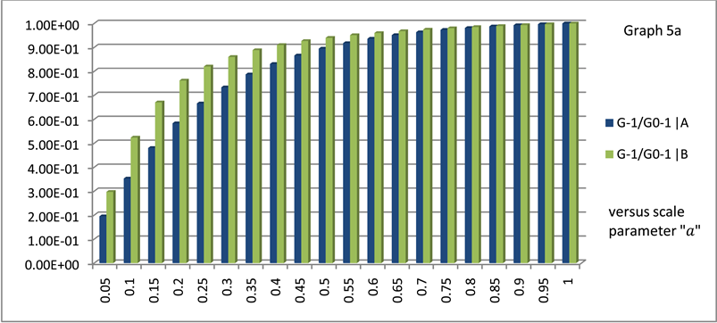Plotting $G^{-1}\left(a\right)$ as a function of “x” gives similar behavior in both models. Graph 5(a) in Appendix C is a preview of the functions plotted as a function of scale parameter “a” up to “a” = 1. Both are well behaved at both high and low temperatures, as we shall see. At very high temperatures in particular, it will be shown that $G^{-1}$ is directly proportional to T in both models, but only in this limiting case.

Using Equation (3-1), we can show that

${\left(G/G_0\right)|}_A=\left(1-{\text{e}}^{-x_0}\right)/\left(1-{\text{e}}^{-x}\right)$ (3-3)

For model B, Equation (3-2) applies and we have correspondingly,

${\left(G/G_0\right)|}_B=\left(\coth \left(x_0\right)-1/x_0\right)/\left(\coth \left(x\right)-1/x\right)=L\left(x_0\right)/L\left(x\right)$ (3-4)

In both equations, it is to be understood that the temperature T marks a particular cosmological epoch. At the onset of $G^{-1}$, we will also have a very specific temperature, which we will call $T_C$, the Curie temperature.

To make progress with these parametrizations, the constant “b” needs to be determined. We know that at present, ${\left(\stackrel{\dot{}}{G}/G\right)|}_0=-0.06H_0$, as is indicated by Equation (2-11). We will use this equality to fix the “b” value for both models A and B. We start with model A. Take the derivative of Equation (3-3) which yields

${\left(G/G_0\right)|}_A=-\left[\left(1-{\text{e}}^{-x_0}\right)/{\left(1-{\text{e}}^{-x}\right)}^2\right]\left({\text{e}}^{-x}\right)\stackrel{\dot{}}{x}$ (3-5)

Divide this by Equation (3-3), left hand side by left hand side, and right hand side by right hand side, to give

${\left(G/G\right)|}_A=-\left[\left({\text{e}}^{-x}\right)/\left(1-{\text{e}}^{-x}\right)\right]\stackrel{\dot{}}{x}=-xH/\left({\text{e}}^x-1\right)$ (3-6)

Remember that $\stackrel{\dot{}}{x}=\stackrel{\dot{}}{a}{x}_0=\left(\stackrel{\dot{}}{a}/a\right)x=Hx$. Next, specialize to the current epoch. In this limit, Equation (3-6) becomes

${\left(\stackrel{\dot{}}{G}/G_0\right)|}_{A0}=-x_0{H}_0/\left({\text{e}}^{x_0}-1\right)$ (3-7)

This can be compared to Equation (2-11), from which it follows that Equation (3-7) can be written as

$-0.06H_0=-x_0{H}_0/\left({\text{e}}^{x_0}-1\right)$ (3-8)

The $H_0$ cancels and a numerical solution can be found to fix the parameter $x_0$. For Equation (3-8) to be satisfied, we must uniquely choose $x_0=4.28$. Hence, $b=x_0{T}_0=4.28\times 2.725=11.663\text{K}$. Summarizing, for model A, we therefore require that

$x_0=4.28,b=11.663\text{K}$ (model A) (3-9)

This fixes our parametrization for model A.

For model B, we proceed similarly. Take the derivative of Equation (3-4) to obtain

${\left(\stackrel{\dot{}}{G}/G_0\right)|}_B=\left[\left(\coth \left(x_0\right)-1/x_0\right)/{\left(\coth \left(x\right)-1/x\right)}^2\right]\left(x{\text{csch}}^{2}x-1/x\right)\stackrel{\dot{}}{x}/x$ (3-10)

We divide the left hand side of Equation (3-10) by the left hand side of Equation (3-4); do the same on the right hand side. In this way we obtain

${\left(\stackrel{\dot{}}{G}/G\right)|}_B=\left[\left(x{\text{csch}}^{2}x-1/x\right)/\left(\coth \left(x\right)-1/x\right)\right]H$ (3-11)

As before, we utilized the identity, $\stackrel{\dot{}}{x}=Hx$. We next specialize (3-11) to the present epoch, which gives

${\left(\stackrel{\dot{}}{G}/G\right)|}_{B0}=\left[\left(x_0{\text{csch}}^2{x}_0-1/x_0\right)/\left(\coth \left(x_0\right)-1/x_0\right)\right]H_0$ (3-12)

We compare this to Equation (2-11). If Equation (2-11) is substituted into (3-12), it turns out that

$-0.06H_0=\left[\left(x_0{\text{csch}}^2{x}_0-1/x_0\right)/\left(\coth \left(x_0\right)-1/x_0\right)\right]H_0$ (3-13)

Again, $H_0$ cancels and a numerical solution can be found. We find that left and right hand sides of Equation (3-13) match if and only if we choose $x_0=17.67$. Thus the “b” in model B has also been uniquely determined because we know that $b=x_0{T}_0=17.67\times 2.725=48.15\text{K}$. Summarizing, for model B

$x_0=17.67,b=48.15\text{K}$ (model B) (3-14)

This determines our parametrization for model B. We note that the temperatures indicated in Equations (3-9) and (3-14) are not particularly high.

We have now specified both functions for $G^{-1}\left(a\right)$. For model A, we use Equation (3-3) with the parameters given in (3-9) substituted. Explicitly,

${\left(G/G_0\right)|}_A=\left(1-{\text{e}}^{-4.28}\right)/\left(1-{\text{e}}^{-4.28a}\right)$ (model A) (3-15)

For model B, we do the same. We use Equation (3-4) with the parameters given in Equation (3-14) substituted. This allows us to write

${\left(\stackrel{\dot{}}{G}/G_0\right)|}_B=\left[\left(\coth \left(17.67\right)-1/17.67\right)/\left(\coth \left(17.67a\right)-1/17.67a\right)\right]$ (model B) (3-16)

For any epoch, G can now be calculated using either Equation (3-15) or (3-16). These functions depend only on the cosmic scale parameter, “a”, or equivalently the CMB temperature.

We next determine $\stackrel{\dot{}}{G}/G$ for both models. For model A, we use Equation (3-6) with $x=a{x}_0=\left(4.28a\right)$ substituted. For model B, we use Equation (3-11) with $x=a{x}_0=\left(17.67a\right)$ substituted. Given any scale factor, we can thus determine a specific value for “x”, and thus find ${\left(\stackrel{\dot{}}{G}/G\right)|}_A$ and ${\left(\stackrel{\dot{}}{G}/G\right)|}_B$ as a function of “a”. We thus have $G/G_0$ and ( $\stackrel{\dot{}}{G}/G$ ) for both models. Equations (3-15) and (3-16) give $G/G_0$. In addition, Equations (3-6) and (3-11), with the appropriate ( $a{x}_0$ ) values substituted, give ( $\stackrel{\dot{}}{G}/G$ ).

Finally, we also wish to calculate the quintessence parameter, w, for models A and B, as well as determine α for models A and B. We know that Equation (2-4) holds. Therefore, it follows that

$\ln \left(G/G_0\right)=-\alpha \ln \left(a\right)$ (3-17)

However, we have specific values for $G/G_0$ as a function of “a”. Hence,

$\alpha =-\ln \left(a\right)/\ln \left(G/G_0\right)\left(G\ne G_0\right)$ (3-18)

Alternatively,

$3\left(1+w\right)=-\ln \left(a\right)/\ln \left(G/G_0\right)\left(G\ne G_0\right)$ (3-19)

Equation (3-18) allows us to determine α as a function of the scale parameter “a”, whereas Equation (3-19) allows us to calculate “w”.

We can now summarize the results. These are presented in table form, Table A1 in Appendix A for various values of “a”. In this table we calculate $G/G_0,\left(\stackrel{\dot{}}{G}/G\right),\alpha$, and w for both models, A and B. The scale parameter is indicated under column 1. The corresponding ${\left(G/G_0\right)|}_A,{\left(G/G_0\right)|}_B,{\left(\stackrel{\dot{}}{G}/G\right)|}_A$, and ${\left(\stackrel{\dot{}}{G}/G\right)|}_B$ values are specified under columns 2, 3, 4 and 5, respectively. The “α” and “w” values are specified under columns 6, 7, 8 and 9. Columns 6 and 7 give the “α” values for models A and B, respectively, whereas columns 8 and 9 are reserved for the “w” values for models A and B, respectively. The table is broken up in four parts. In part one, we cover the range where “a” equals 1 through to 0.1. In part two, “a” values in the range 0.1 to 0.01 are considered. In part three, “a” is allowed to run through the values from 0.01 to 0.001. In addition, in part four, we consider future values for “a”. In this part, “a” will start at 1 and move up to 10, in increments of one unit per row. So, in the first three parts, we are going progressively back in cosmological time, whereas in the 4^th part, we are moving forward in time, cosmologically speaking.

We also present graphs for the quantities calculated above. These illustrations are given in Appendix B, and the values correspond to the entries specified in Table A1. We present the graphs in a certain order. First model A is always compared with model B, quantity with corresponding quantity. This is done such that we can visually compare the difference between models A and B. On the horizontal axis, we always plot the scale parameter “a”. On the vertical axis, we plot $G/G_0$, $\left(\stackrel{\dot{}}{G}/G\right)$, “α” and “w” for both models A and B. Graphs 1(a)-(d) give these values for “a” in the range from 1 to 0.1. Graphs 2(a)-(d) do the same for “a” values in the range from 0.1 and 0.01. Graphs 3(a)-(d) are reserved for “a” values in the range from 0.01 to 0.001. And finally, Graphs 4(a)-(d) give the values outlined above for “a” in the range from 1 to 10. Therefore, Graph 1 refer to part 1 in the table, Graph 2 refer to part 2 in the table, Graph 3 to part 3 in the table, and Graph 4 refer to part 4 in the table.

Upon comparing the numerical values between models A and B, we notice a remarkable similarity. Model B is somewhat more conservative in that $G/G_0$ does not increase quite as dramatically as in model A when we go back in time towards higher temperatures. Nevertheless, the order of magnitude estimates seem to be on a par right up to and including the very early universe. Both models lead to essentially the same results, even though the two parametrizations are distinct from each other. We remark that these functionalities for $G^{-1}$ in terms of “a” depends critically on our original choice for w, namely that specified by Equation (1-1). This determined Equation (2-11), which furthermore allowed us to fix the parameter “b” in both models. If we had chosen a value closer to −1 for w, then there would be little to no difference between the ΛCDM concordance model, and our models A and B. Our parametrizations deviate from the ΛCDM model precisely because we do not set w equal to −1, a-priori. A higher or lower value for “w” at present will dramatically affect the evolution of $G/G_0$.

We also note that in the limit of low T, the “w” values automatically approach −1, and α approaches zero. Thus, the ΛCDM model is approached in both our models in the low temperature limit. At very high temperatures, on the other hand, the quintessence parameter, w, approaches a value of −2/3 in both models. This will give a value for α equal to unity.

Both models A and B have the correct limits for an order parameter, $G^{-1}\left(a\right)$. This we will now show. First, quite generally, irrespective of the model employed, it is to be noticed that the following general identity holds:

$\text{d}/\text{d}t\left(G^{-1}\right)/G^{-1}=-G^{-2}\stackrel{\dot{}}{G}/G^{-1}=-\stackrel{\dot{}}{G}/G$ (3-20)

Upon using Equation (3-20), it is straightforward to show that

$\text{d}/\text{d}t\left(G^{-1}\right)/\left(G^{-1}\right)=-\stackrel{\dot{}}{G}/G=xH/\left({\text{e}}^x-1\right)$ (model A) (3-21)

And, for model B,

$\text{d}/\text{d}t\left(G^{-1}\right)/\left(G^{-1}\right)=-\stackrel{\dot{}}{G}/G=-\left[\left(x{\text{csch}}^{2}x-1/x\right)/\left(\coth x-1/x\right)\right]H$ (model B) (3-22)

In Equation (3-21), we have made use of equations (3-6). In addition, for Equation (3-22), Equation (3-11) was employed.

We can consider the limit where $a\to 0$. In this limit, $x\equiv \left(a{x}_0\right)\to 0$. Therefore, for small values of x, ${\text{e}}^x\cong \left(1+x\right)$, and Equation (3-21) reduces to

$\lim a\to 0\text{d}/\text{d}t\left(G^{-1}\right)/\left(G^{-1}\right)=H$ (model A) (3-23)

A similar result holds for Equation (3-22). For small values of x, a power series expansion yields

$\left(x{\text{csch}}^{2}x-1/x\right)=-x/3+x^3/15-2x^5/189+\cdots$ (3-24a)

$\left(\coth x-1/x\right)=x/3-x^3/45+2x^5/945+\cdots$ (3-24b)

Keeping only terms to first order in x, Equation (3-22) reduces to

$\lim a\to 0\text{d}/\text{d}t\left(G^{-1}\right)/\left(G^{-1}\right)=H$ (model B) (3-25)

In this limit of very small “a”, it is clear that $\text{d}\left(G^{-1}\right)/\left(G^{-1}\right)=\text{d}a/a=-\text{d}T/T$, for both models, A and B. At very high temperatures, i.e., very low “a” values, it follows that $\left(G_1^{-1}/G_2^{-1}\right)=G_2/G_1=a_1/a_2=T_2/T_1$.

The other extreme is the limit where $a\to \infty$, which means going forward in time starting from the present epoch. In this interesting case, the reader will notice that the entries in our Table 1 indicate a saturation value for both models A and B. In fact, as can be read off the table (see the entries under columns 2 and 3), we find in the limit of large “a”

${\left(G_{\infty }\right)|}_A=0.986G_0$ (model A; large “a”) (3-26)

${\left(G_{\infty }\right)|}_B=0.949G_0$ (model B; large “a”) (3-27)

Hence,

${\left(G_{\infty }^{-1}\right)|}_A=1.014G_0^{-1}$ (model A; large “a”) (3-28)

${\left(G_{\infty }^{-1}\right)|}_B=1.054G_0^{-1}$ (model B; large “a”) (3-29)

These are the saturation values to be used in equations (3-1) and (3-2), respectively. At present, $G^{-1}$ is varying very slowly because we are already close to saturation. The value $G^{-1}$ will eventually stop increasing in both models. For model A, this occurs already at roughly $a\approx 2$. For model B, $G^{-1}$ becomes virtually a constant at $a\approx 10$. See table I, and the graphs given in Appendix B, specifically Graph 4(a) and Graph 4(b). We are late in the evolution of $G^{-1}$ in the present epoch, and Newton’s constant, $G_0$, will not decrease much further as indicated by equations (3-26) and (3-27). These are the saturated limits for Newton’s constant as calculated by our models.

Before we leave this section, we give another table, Table C1 in Appendix C. Here we calculate $G^{-1}/G_0^{-1}$, and $\left\{\text{d}\left(G^{-1}\right)/\text{d}t\right\}/G^{-1}$ as a function of “a”, but moving forward in time starting in the distant past. We start with “a” = 0.05 and work our way up to the present day where “a” = 1. This is more natural as we are proceeding from higher energies to lower ones, from a time in the distant past to the present. Keep in mind that $G^{-1}$ is our order parameter, and not G. For $G^{-1}$, we use Equations (3-1) and (3-2) with the parameters (3-9) and (3-14) substituted, respectively. Equations (3-1) with (3-9) hold for model A while Equations (3-2) with (3-14) hold for model B. Furthermore, we can make use of Equation (3-20) for $\left\{\text{d}\left(G^{-1}\right)/\text{d}t\right\}/G^{-1}$. 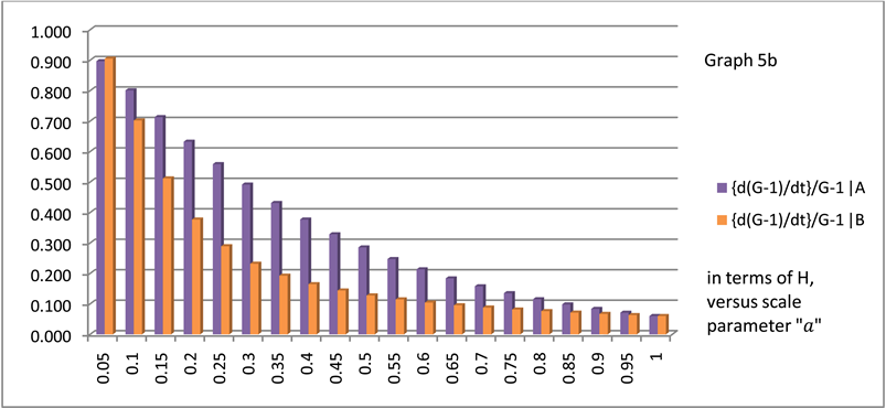This is given in units of H, Hubble’s parameter. This is just another way of representing what was said thus far. However, in this formulation, we clearly see the evolution of the inverse Newtonian constant, our order parameter. There is a difference between the specific evolutions for models A and B.

We highlight this difference between models A and B more explicitly using graphs. In Appendix C, we present two graphs, Graph 5(a) and Graph 5(b). Graph 5(a) gives $G^{-1}/G_0^{-1}$ for both our models, A and B. Graph 5(b), on the other hand, gives $\left\{\text{d}\left(G^{-1}\right)/\text{d}t\right\}/G^{-1}$ for both models, in units of H. In both models, as $G^{-1}/G_0^{-1}$ increases, $\left\{\text{d}\left(G^{-1}\right)/\text{d}t\right\}/G^{-1}$ decreases. At present, $\left\{\text{d}\left(G^{-1}\right)/\text{d}t\right\}/G^{-1}$ hardly changes at all. Again, this is just another way of presenting what was determined previously.

4. Cosmic Time Evolution for G⁻¹⁽a)

In the conventional picture, the ΛCDM model where $\stackrel{\dot{}}{G}/G=0$ and $w=-1$, we know that $a\left(t\right)$ is proportional to t^1/2 for a radiation dominated universe, $a\left(t\right)$ is proportional to t^3/2 for a matter dominated universe, and $a\left(t\right)$ is proportional to ${\text{e}}^{Ht}$ for a dark energy dominated universe. If $\stackrel{\dot{}}{G}/G\ne 0$, however, the time dependency is more complicated. This we now consider.

To be specific, we resort to our two parametrizations, model A and model B given by Equations (3-1 and (3-2), respectively. First we review the steps in the ΛCDM model where $\stackrel{\dot{}}{G}/G=0$,and $w=-1$. Utilizing Equation (2-2), and recognizing that $H=\stackrel{\dot{}}{a}/a$, we can see that

$\stackrel{\dot{}}{a}/a=H_0{\left({\Omega }_{RAD}{a}^{-4}+{\Omega }_{MATTER}{a}^{-3}+{\Omega }_{\Lambda }\right)}^{\frac{1}{2}}$ (4-1)

Thus

$\text{d}t=H_0^{-1}{\left({\Omega }_{RAD}{a}^{-4}+{\Omega }_{MATTER}{a}^{-3}+{\Omega }_{\Lambda }\right)}^{-\frac{1}{2}}\text{d}a/a$ (4-2)

Integrating gives

$\left(t_0–t\right)=H_0^{-1}{\displaystyle {\int }_a^1{\left({\Omega }_{RAD}{a}^{-4}+{\Omega }_{MATTER}{a}^{-3}+{\Omega }_{\Lambda }\right)}^{-\frac{1}{2}}\text{d}a/a}$ (4-3)

In Equation (4-3), $\left(t_0–t\right)$ is the look-back time. Setting $t=0$ corresponds to going back to the beginning of cosmological time, where $a=0$. If we go forward in time, we can define a look-forward time where the limits of integration are reversed, and the left hand side is replaced by $\left(t_0–t\right)$. Both integrals are performed using numerical integration once the ${\Omega }_{RAD},{\Omega }_{MATTER}$ _, and ${\Omega }_{\Lambda }$ values have been substituted. In the above equation, we can take $H_0$ equal to

$67.74\text{km}/\left(\text{s}\cdot \text{Mpc}\right)=2.195\times {10}^{-18}{\text{s}}^{-1}={\left(14.44\times {10}^9\right)}^{-1}{\text{yr}}^{-1}$, andthe density parameters can be chosen as $\left({\Omega }_{RAD},{\Omega }_{MATTER},{\Omega }_{\Lambda }\right)=\left(8.3\times {10}^{-5},0.3089,0.6911\right)$. This would conform to the parameters suggested by the Planck VIII collaboration. Equation (4-3) will give us precisely the age of the universe, $t_0=13.8\text{Gyr}$, if we set $t=0$ on the left hand side and “a” = 0 on the right.

We note that in the very early universe, radiation dominates due to the high value of $a^{-4}$. In this instance, the second and third terms on the right hand side of Equation (4-3) are negligible, and we obtain the customary t^1/2 dependency for $a\left(t\right)$ at high temperatures. For a matter-dominated universe, the ${\Omega }_{MATTER}$ term dominates in Equation (4-3), because the first and third terms are small for intermediate “a” values. Here it is easy to show that $a\left(t\right)$ is proportional to t^3/2. Finally, for a dark energy dominated universe, the third term takes over within the integral of Equation (4-3). In this instance, we have a ${\text{e}}^{Ht}$ dependency for $a\left(t\right)$. In Table C1, column 2, in Appendix C we have calculated specific look-back times as well as look-forward times for the ΛCDM model as a function of scale parameter, “a”, which is indicated in column 1. We made use of equations (4-3) with the density parameter coefficients inserted. Numerical integration was performed using an on-line integrator, integral-calculator.com.

For models A and B, both Equations (4-2) and (4-3) are modified. For model A, the counterpart to Equation (4-3) is

$\left(t_0–t\right)=H_0^{-1}{\displaystyle {\int }_x^{x_0}{\left[\left(1-{\text{e}}^{-x}\right)/\left(1-{\text{e}}^{-x_0}\right)\right]}^{\frac{1}{2}}{\left({{\Omega }^{\prime }}_{RAD}{x}^{-2}+{{\Omega }^{\prime }}_{MATTER}{x}^{-1}+{\Omega }_{\Lambda }{x}^2\right)}^{-1/2}\text{d}x}$ (4-4)

To show this we start with Equation (3-3). We substitute Equation (3-3) into Equation (2-12) to obtain

$\stackrel{\dot{}}{a}/a=H_0{\left[\left(1-{\text{e}}^{-x_0}\right)/\left(1-{\text{e}}^{-x}\right)\right]}^{\frac{1}{2}}{\left({\Omega }_{RAD}{a}^{-4}+{\Omega }_{MATTER}{a}^{-3}+{\Omega }_{\Lambda }\right)}^{\frac{1}{2}}$ (4-5)

From this, it follows that

$\text{d}t=H_0^{-1}{\left[\left(1-{\text{e}}^{-x}\right)/\left(1-{\text{e}}^{-x_0}\right)\right]}^{1/2}{\left({\Omega }_{RAD}{a}^{-4}+{\Omega }_{MATTER}{a}^{-3}+{\Omega }_{\Lambda }\right)}^{-1/2}\text{d}a/a$ (4-6)

However, recall that $x=a{x}_0$. Therefore $\text{d}x=\text{d}a{x}_0$ and $\text{d}a/a=\text{d}x/x$. Furthermore $a^{-4}={\left(x/x_0\right)}^{-4}$, and $a^{-3}={\left(x/x_0\right)}^{-3}$. We redefine ${\Omega }_{RAD},{\Omega }_{MATTER}$ as ${{\Omega }^{\prime }}_{RAD},{{\Omega }^{\prime }}_{MATTER}$, where

${{\Omega }^{\prime }}_{RAD}\equiv {\Omega }_{RAD}{x}_0^4=\left(8.3\times {10}^{-5}\right){\left(4.28\right)}^4=0.02785$ (4-7a)

${{\Omega }^{\prime }}_{MATTER}\equiv {\Omega }_{MATTER}{x}_0^3=\left(0.3089\right){\left(4.28\right)}^3=24.2186$ (4-7b)

This allows us to rewrite Equation (4-6) as

$\begin{array}{l}\text{d}t=H_0^{-1}{\left[\left(1-{\text{e}}^{-x}\right)/\left(1-{\text{e}}^{-x_0}\right)\right]}^{1/2}{\left({{\Omega }^{\prime }}_{RAD}{x}^{-4}+{{\Omega }^{\prime }}_{MATTER}{x}^{-3}+{\Omega }_{\Lambda }\right)}^{-1/2}\text{d}x/x\\ =H_0^{-1}{\left[\left(1-{\text{e}}^{-x}\right)/\left(1-{\text{e}}^{-x_0}\right)\right]}^{\frac{1}{2}}{\left({{\Omega }^{\prime }}_{RAD}{x}^{-2}+{{\Omega }^{\prime }}_{MATTER}{x}^{-1}+{\Omega }_{\Lambda }{x}^2\right)}^{-\frac{1}{2}}\text{d}x\end{array}$ (4-8)

Equation (4-4) follows from relation (4-8). Since $x_0=4.28$, we can evaluate the constant, ${\left(1-{\text{e}}^{-x_0}\right)}^{1/2}=0.9931$.

For model B, the analogue of Equation (4-3) is

$\begin{array}{c}\left(t_0–t\right)=H_0^{-1}{\displaystyle {\int }_x^{x_0}{\left[\left(\coth \left(x\right)-1/x\right)/\left(\coth \left(x_0\right)-1/x_0\right)\right]}^{\frac{1}{2}}}\\ \times {\left({{\Omega }^{\prime }}_{RAD}{x}^{-2}+{{\Omega }^{\prime }}_{MATTER}{x}^{-1}+{\Omega }_{\Lambda }{x}^2\right)}^{-\frac{1}{2}}\text{d}x\end{array}$ (4-9)

We follow the same steps as before. We start with Equation (3-4) and substitute this into Equation (2-12). This gives

$\stackrel{\dot{}}{a}/a=H_0{\left[\left(\coth \left(x_0\right)-1/x_0\right)/\left(\coth \left(x\right)-1/x\right)\right]}^{\frac{1}{2}}{\left({\Omega }_{RAD}{a}^{-4}+{\Omega }_{MATTER}{a}^{-3}+{\Omega }_{\Lambda }\right)}^{\frac{1}{2}}$ (4-10)

From this, it follows that

$\begin{array}{c}\text{d}t=H_0^{-1}{\left[\left(\coth \left(x\right)-1/x\right)/\left(\coth \left(x_0\right)-1/x_0\right)\right]}^{1/2}\\ \times {\left({\Omega }_{RAD}{a}^{-4}+{\Omega }_{MATTER}{a}^{-3}+{\Omega }_{\Lambda }\right)}^{-1/2}\text{d}a/a\end{array}$ (4-11)

However, we know that $\text{d}a/a=\text{d}x/x$. Also, $a^{-4}={\left(x/x_0\right)}^{-4}$ and $a^{-3}={\left(x/x_0\right)}^{-3}$, as before. If we redefine our density parameters as follows:

${{\Omega }^{\prime }}_{RAD}\equiv {\Omega }_{RAD}{x}_0^4=\left(8.3\times {10}^{-5}\right){\left(17.67\right)}^4=8.0914$ (4-12a)

${{\Omega }^{\prime }}_{MATTER}\equiv {\Omega }_{MATTER}{x}_0^3=\left(0.3089\right){\left(17.67\right)}^3=1.7042\times {10}^3$ (4-12b)

then we can rewrite Equation (4-11) as

$\begin{array}{c}\text{d}t=H_0^{-1}{\left[\left(\coth \left(x\right)-1/x\right)/\left(\coth \left(x_0\right)-1/x_0\right)\right]}^{\frac{1}{2}}\\ \times {\left({{\Omega }^{\prime }}_{RAD}{x}^{-2}+{{\Omega }^{\prime }}_{MATTER}{x}^{-1}+{\Omega }_{\Lambda }{x}^2\right)}^{-\frac{1}{2}}\text{d}x\end{array}$ (4-13)

From this equation, it is clear how Equation (4-9) follows. Since $x_0=17.67$, we can work out the constant in Equation (4-13), namely, ${\left(\coth \left(x_0\right)-1/x_0\right)}^{1/2}=0.9713$. As always, to obtain the look-forward times, we reverse the limits of integration in both Equations (4-4) and (4-9), and substitute for the left hand side, $\left(t–t_0\right)$.

Now that we have Equation (4-4) for model A, and correspondingly, Equation (4-9) for model B, we can numerically evaluate the integrals. All coefficients are known except for x. The limits of integration for model A, are from $x=\left(a{x}_0\right)=\left(4.28a\right)$ to $x_0=4.28$. This is to be used with Equation (4-4). For model B, we use Equation (4-9) where the limits are from $x=\left(a{x}_0\right)=\left(17.67a\right)$ to $x_0=17.67$. The results of the numerical integrations are specified in Table D1 in Appendix D, under columns 3 and 4. These are calculated as a function of scale parameter “a”, which is given under column 1. Column 3 holds for model A, and column 4 is valid for model B. These values can be compared to those values for the ΛCDM model, which we have listed under column 2. Upon comparison of the numerical results, most values of “a” give similar results. It is only when one gets to relatively low “a” values where one notices a real deviation.

A graph comparing the three models is illustrated in Graph 6(a). One glaring difference between the models is the predicted age of the universe. The ΛCDM model gives a predicted age of $0.9559H_0^{-1}=0.9559\left(14.44\text{Gyr}\right)=13.8\text{Gyr}$. Model A, by contrast, predicts a naïve value equal to $t_0=0.8688H_0^{-1}=0.8688\left(14.44\text{Gyr}\right)=12.5\text{Gyr}$. Moreover, model B predicts a third value equal to $t_0=0.9018H_0^{-1}=0.9018\left(14.44\text{Gyr}\right)=13.0\text{Gyr}$. Quite generally, the age of the universe is given by the expression, $t_0=F\left({\Omega }_{RAD},{\Omega }_{MATTER},{\Omega }_{\Lambda }\right)\ast H_0^{-1}$, where F is the so-called “age correction factor” [14] . The function, F, is specifically what we are plotting in Graph 6(a). Its value depends on the density parameters chosen. Since we have made a specific choice, the value for F is determined as specified above. The age correction factors are (0.9559, 0.8688, 0.9018) for the (ΛCDM, Model A, Model B) models, respectively, if we adopt i.e., accept ${\Omega }_{RAD}=0.000083$, ${\Omega }_{MATTER}=0.3089$, and ${\Omega }_{\Lambda }=0.6911$ as our input values. Seeing that the predicted ages of the universe in models A and B seem low, we have several options:

a) $H_0^{-1}$ has to be adjusted

b) The values for ${\Omega }_{RAD}$, ${\Omega }_{MATTER}$, and ${\Omega }_{\Lambda }$ have to be changed

c) The age is as specified, i.e., the universe is less than 13.8 Gyr old

d) Some combination of the above. (4-14)

We will discount option c) as the 13.8 Gyr age seems to be a well-established fact. The age of the oldest globular clusters certainly indicate an age in excess of 12.5 Gyr. The analysis of the acoustic peaks in WMAP and Planck satellite data also seem to preclude a lessor age for the universe. Therefore, we will discount option c). We will also ignore option d) as we are focused on most likely principle sources. This leaves options a) or b).

Option b) would require adopting a new set of values for ${\Omega }_{MATTER}$ and ${\Omega }_{\Lambda }$, other than the 0.3089 and 0.6911 respective values chosen. The ${\Omega }_{RAD}=0.000083$ value is not that critical for the numerical age determination of the universe. Adjusting ${\Omega }_{MATTER}$ and ${\Omega }_{\Lambda }$ values is a distinct possibility; it means changing the values towards a higher dark energy component, and a lessor dark matter contribution. Hence, we would be apt to dismiss option b) as well. However, we remark that if we had made a different choice for model A, namely, ${\Omega }_{MATTER}=0.212$, and ${\Omega }_{\Lambda }=0.788$, then the correction factor would match that of the ΛCDM result, namely, 0.9559. For model B, if we adjust ${\Omega }_{MATTER}$ to equal 0.249 with ${\Omega }_{\Lambda }$ equaling 0.751, then we would also match the ΛCDM correction factor exactly without any need for further fine-tuning. If we do not wish to change the values of the density parameters as determined by the Planck VIII collaboration, this leaves option a) as our best option.

Working within the framework of option a), we adjust our $H_0^{-1}$ values accordingly such that we reproduce 13.8 Gyr as the age of the universe. For model A, we demand specifically that

$0.9559H_0^{-1}=0.8688H_{0A}^{-1}$ (4-15)

where $H_{0A}$ is the value of the Hubble constant to be used for model A, and $H_0=67.74\text{km}/\left(\text{s}\cdot \text{Mpc}\right)$, the specified value as determined by the 2015 Planck XIII cosmological parameter collaboration. Solving Equation (4-15) gives us a value for $H_{0A}^{-1}$ ; it is

$H_{0A}^{-1}=15.99\text{Gyr}\text{or}{H}_{0A}=61.7\text{km}/\left(\text{s}\cdot \text{Mpc}\right)$ (4-16)

For model B, likewise, we can demand that

$0.9559H_0^{-1}=0.9018H_{0B}^{-1}$ (4-17)

where $H_{0B}$ is the value of Hubble’s constant to be employed for model B, and $H_0$ is the established value as determined by the 2015 Planck XIII collaboration. Solving Equation (4-17) gives a value for $H_{0B}^{-1}$. We obtain in this instance,

$H_{0B}^{-1}=15.3\text{Gyr}\text{or}{H}_{0B}=63.9\text{km}/\left(\text{s}\cdot \text{Mpc}\right)$ (4-18)

The values indicated in Equations (4-16) and (4-18) may seem low. However, we believe that they are entirely within of the range of observations.

We believe that these values for $H_{0A}$ and for $H_{0B}$ can be justified because $H_0$ is not that well determined, observationally. In fact, as of 2015, there is still a range of values, which can be assigned to $H_0$. As noted in reference [14] , the Planck 2015 XIII cosmological parameter collaboration, there is a noted discrepancy (referred to as “tension”) between the 9 year WMAP determination of $H_0$ and the newer Planck satellite limit on $H_0$. The latest Planck determination for $H_0$ is less than that determined previously by WMAP. Furthermore, analyzing other data, such as Cepheid Variables, give limits for $H_0$ as high as [41] $74.3\pm 2.6\text{km}/\left(\text{s}\cdot \text{Mpc}\right)$ [Friedmann] [et al. 2012] and as low as [42] $63.7\pm 2.3\text{km}/\left(\text{s}\cdot \text{Mpc}\right)$ [Tammann & Reindl] [2013]. These are not to be ruled out. The latter limit is interesting because both our models A and B fall clearly within this range. Model B is almost a perfect match, whereas model A is within the lower limit. Hence, if we normalize $H_0$ appropriately as was done in Equations (4-14) and (4-16), then we believe we can keep the 13.8 Gyr age of the universe intact, and still stay within our model parametrizations. No revision in either ${\Omega }_{MATTER}$ or ${\Omega }_{\Lambda }$ is needed. The normalized results for models A and B are presented in Table D2 of Appendix D. The corresponding graph is given in Graph 6(b). Upon comparison of the entries in columns 3 and 4 with those of column 2, the ΛCDM model, we see agreement. Models A and B indicate slightly larger look-back times in the latter epochs (large “a”). Nevertheless, eventually, the ΛCDM model catches up with the same look-back times at a lower “a”. We speculate that the larger look-back times in the latter epochs give the unanticipated acceleration of the universe. Ultimately, it is connected to a weakening G in the latter epochs.

We close this section by noting that if we wish to compare look-back times between models A and B, and ΛCDM, it may turn out that “w” has a different value at present than the one selected, which was $w_0=-0.98$. This is almost certainly true if space is not flat. If space is curved, then instead of using Equation (1-1) for w, we should be using Equation (1-2), or some variation thereof, as our approximation for “w”. Moreover, if we accept the value for “w” listed in (1-2), then it would be very difficult to differentiate our models A and B from the ΛCDM model. In fact, our models A and B would be almost identical to the ΛCDM model in terms of predictions because “w” is so close to −1. For other “w” values in a flat space, the look-back times would also have to be re-worked. We bring this up only to show that there is greater flexibility than is indicated by our conditions (4-14), in either dismissing or accepting a variable G assumption given a specified age.

5. Estimating the Onset of Gravity, at $G^{-1}=G^{-1}(aC)$

Our parametrizations, given by Equations (3-1) and (3-2), assume that $G^{-1}\left(a\right)$ is an order parameter, which approaches a constant value at low energies, i.e., at low CMB temperatures. The values measured today for $G_0$ are fairly close to those constant saturation values, $G_{\infty }$, as is indicated by Equations (3-28) and (3-29). This can also be seen in Graph 5(a) in Appendix C where a saturation value is clearly visible. At some time in the distant past, however, at low enough “a”, i.e., at sufficiently high CMB temperatures, $G^{-1}$ must have come into existence. In other words, gravity, as we know it, must have emerged. A small value for $G^{-1}$ must mean a large value for G. This ansatz was specifically introduced to solve the cosmic vacuum fine-tuning problem. See the discussion around Equation (2-23). The big question now arises: can we estimate the onset of $G^{-1}$? Can we give a specific temperature, or equivalently, a specific cosmic scale, for G formation? We will call the critical temperature for G formation, $T_C=T\left(a_C\right)$, where $a_C$ is the scale parameter at inception of $G^{-1}$. $G\left(a_C\right)$ is thus the same as $G\left(T_C\right)$ because of the relation between scale parameter and CMB temperature, $a={\left(1+z\right)}^{-1}=T_0/T$.

To answer this question, we first consider the Planck scale. At this scale, we supposedly have super grand unification where gravity, thermodynamics, and quantum mechanical fluctuations create a so-called “quantum foam” where virtual particles constantly interact and exchange energy with the underlying space-time continuum, producing a turbulent vacuum froth. Neither space-time nor matter/energy will have a clear identity under those conditions. This is also the scale where our knowledge of physics breaks down because we cannot say anything intelligent beyond it, energy wise. The Planck scale invariably involves Newton’s constant, G. In fact, the Planck length, the Planck time, the Planck mass, the Planck energy, etc., are all defined explicitly in terms of G. To be specific, we note that the Planck length, $L_P\equiv {\left(ћG/c^3\right)}^{1/2}=1.62\times {10}^{-35}\text{m}$. The Planck mass is given by $M_P\equiv {\left(ћc/G\right)}^{1/2}=2.18\times {10}^{-8}\text{kg}$. The Planck time is defined as $t_P\equiv {\left(ћG/c^5\right)}^{1/2}=5.39\times {10}^{-44}\text{s}$. We have the Planck energy,

$E_P\equiv {\left(ћc^5/G\right)}^{1/2}=1.96\times {10}^9\text{J}=1.225\times {10}^{19}\text{GeV}$. Then there is the Planck tem-

perature, $T_P\equiv {\left(ћc^5/G{k}_B^2\right)}^{1/2}=1.42\times {10}^{32}\text{K}$, etc. We see that all are defined in terms of G, Newton’s constant. The notable exception is the Planck charge, $q_P\equiv {\left(4\text{π}{\epsilon }_0ћc\right)}^{1/2}=1.88\times {10}^{-18}\text{Coulombs}$, which, interestingly, does not involve G explicitly. However, if G is not fundamental, then it can be argued that neither is the Planck scale. In fact, if we believe gravity to be a low energy phenomenological limit, then there is nothing significant about the Planck scale.

Nevertheless, there is one relationship in the above, which can prove useful. That is the Planck temperature, $T_P\equiv {\left(ћc^5/G{k}_B^2\right)}^{1/2}$. Instead of $T_P$, we replace the left hand side by $T_C$, the Curie temperature, which will signify the onset of gravity. Moreover, on the right hand side we recognize that G is also temperature dependent. This means that at the formation of G, we must have

$T_C\equiv {\left(ћc^5/G_C{k}_B^2\right)}^{1/2}$ (5-1)

In this expression, the gravitational “constant” becomes $G_C=G\left(T_C\right)=G\left(T_0/a_C\right)$. Equation (5-1) is a necessary requirement for consistency at a high enough temperature.

Now, for model A at very high temperatures, i.e., very low “a” values, we know that we can approximate Equation (3-3) by

$\begin{array}{l}G=G_0\left[\left(1-{\text{e}}^{-x_0}\right)/\left(1-{\text{e}}^{-a{x}_0}\right)\right]\\ =G_0\left[\left(1-{\text{e}}^{-x_0}\right)/\left(a{x}_0\right)\right]\\ =G_0\left[\left(1-{\text{e}}^{-x_0}\right)T/\left(T_0{x}_0\right)\right]\left(x\ll 1\right)\end{array}$ (5-2)

At inception of $G^{-1}$, $T_C$ replaces the temperature T. We can also substitute the values specified in Equation (3-9). Inserting both into Equation (5-2) allows us to write that at G formation,

$G_C=0.08455G_0{T}_C$ (model A) (5-3)

For model B, at very high temperatures, i.e., very small “a” values, Equation (3-4) can also be approximated. In this instance,

$\begin{array}{l}G=G_0\left[\left(\coth \left(x_0\right)-1/x_0\right)/\left(\coth \left(x\right)-1/x\right)\right]\\ =G_{0}3\left[\left(\coth \left(x_0\right)-1/x_0\right)/\left(x\right)\right]\\ =G_{0}3T\left[\left(\coth \left(x_0\right)-1/x_0\right)/\left(T_0{x}_0\right)\right]\left(x\ll 1\right)\end{array}$ (5-4)

Again, G is proportional to T, just as in Equation (5-2), for very small “x”. In the second line of Equation (5-4), use has been made of the fact that for small x, the Langevin function reduces to $L\left(x\right)\equiv \coth \left(x\right)-1/x\cong x/3$. At inception of $G^{-1}$, $T_C$ replaces T. Furthermore, we can insert our values specified by Equation (3-14). Substituting both into Equation (5-4) gives in this situation

$G_C=0.0587G_0{T}_C$ (model B) (5-5)

We emphasize that for both models A and B, G is proportional to T. Hence, $G_C$ is directly proportional to $T_C$. This holds only in the limit of small x, or equivalently, small “a” values (very high temperatures). It must therefore hold true at temperature, $T=T_C$.

We next substitute Equations (5-3) and (5-5) into our fundamental relation, Equation (5-1). We start with Equation (5-3). Substituting this into relation (5-1) gives

$T_C\equiv {\left(ћc^5/G_0{k}_B^2\right)}^{1/2}{\left(0.08455T_C\right)}^{-1/2}=1.42\times {10}^{32}{\left(0.08455T_C\right)}^{-1/2}$ (5-6)

Solving for $T_C$, we find

$T_C=6.20\times {10}^{21}\text{K}$ (model A) (5-7)

For model B, we proceed analogously. We substitute Equation (5-5) into Equation (5-1). In this instance, we obtain

$T_C\equiv {\left(ћc^5/G_0{k}_B^2\right)}^{1/2}{\left(0.0587T_C\right)}^{-1/2}=1.42\times {10}^{32}{\left(0.0587T_C\right)}^{-1/2}$ (5-8)

Solving for $T_C$, we find

$T_C=7.01\times {10}^{21}\text{K}$ (model B) (5-9)

The values obtained for $T_C$ in models A and B are numerically very close to one another. The values are within a percentage of each other. The temperatures are large, but still very well below the Planck temperature, which equals $1.42\times {10}^{32}\text{K}$. In fact, in retracing our steps, we find that we can approximate $T_C$ for both models A and B as $T_C\approx {\left(T_P\right)}^{2/3}$. The temperature, $T_C$ _, is fundamental in our view whereas the Planck temperature, $T_P$, on the other hand, is not.

The associated scale for $G^{-1}$ formation is given next. For models A and B, using our temperatures (5-7) and (5-9), we find that

$a_C=T_0/T_C=4.37\times {10}^{-22}$ (model A) (5-10a)

$a_C=T_0/T_C=3.89\times {10}^{-22}$ (model B) (5-10b)

Because the $T_C$ values are very close in both models, it comes as no surprise that the “ $a_C$ “ values are very close as well. The redshift at G formation is very high if we accept the scale factor determinations specified in Equation (5-10).

In Table E1 in Appendix E, we have specified the scale parameters indicated by Equations (5-10a) and (5-10b). We have also calculated accordingly the $G/G_0$ values at these scales, as well as other quantities, given our formulae above. For the two models presented, the values calculated are

$G/G_0=5.273\times {10}^{20}$ (model A) (5-11a)

$G/G_0=4.113\times {10}^{20}$ (model B) (5-11b)

We see that both values are close to one another in magnitude and quite large. We believe that there could very well be a twenty order of magnitude increase in G at these extremely high temperatures. At “a” = 0.001 which is close to recombination, G is still comparatively low in value, and that already puts us at a look-back time of 13.8 Gyr. For model A, $G/G_0$ equals 231, whereas for model B, $G/G_0=160$, for a cosmic scale equal to “a” = 0.001. See Table A1 in Appendix A. However, we are dealing with much higher temperatures at 10²¹ K, and at this temperature, the ratio $G/G_0$ is certainly much larger. Again, this would go a long way towards explaining the vacuum energy discrepancy between present and past values.

The cosmological constant, Λ, is sometimes referred to as the “mass of the vacuum”. Due to our Equation (2-23), we can estimate its value at G formation. We substitute Equations (5-11a) and (5-11b) into relations (2-23). This gives

$\Lambda /{\Lambda }_0=2.78\times {10}^{41}$ (model A) (5-12a)

$\Lambda /{\Lambda }_0=1.69\times {10}^{41}$ (model B) (5-12b)

We do not have the 122 order of magnitude difference between present and past values because we are stopping well short of the Planck scale. We have instead a 41 order of magnitude increase, as indicated by Equations (5-12a) and (5-12b). Dark energy does scale in our estimation, but never by nearly as much as either matter or radiation. The most radical scaling of dark energy occurs in the very early universe as it is there that the “w” values deviate significantly from minus one.

It has been argued that gravity may not be a fundamental force. Instead it may a low energy phenomenological limit which vanishes at incredibly high temperatures/energies, at the scales indicated by Equations (5-7) and (5-9). If this is the case, then it would be interesting to calculate the radiative energy density, the dominant form of energy at these very high temperatures. Using Planck’s formula, $u=4\sigma T^4/c$ where σ = Stefan-Boltzmann constant $=5.67\times {10}^{-8}\text{J}/\left(\text{s}\cdot {\text{m}}^{\text{2}}\cdot {\text{K}}^{\text{4}}\right)$, we find that for model A we have an energy density of the order $u\left(T_C=6.20\times {10}^{21}\text{K}\right)=1.12\times {10}^{72}\text{J}/{\text{m}}^{\text{3}}$. For model B, we have correspondingly, $u\left(T_C=7.01\times {10}^{21}\text{K}\right)=1.83\times {10}^{72}\text{J}/{\text{m}}^{\text{3}}$. While high, they are nowhere near as large as those which one would obtain at a Planck temperature of $T_P=1.42\times {10}^{32}\text{K}$. In that instance, the energy density works out to equal $u=3.07\times {10}^{113}\text{J}/{\text{m}}^{\text{3}}$. For radiation, the pressure is always one-third the energy density. Therefore, at formation temperatures of approximately $6\times {10}^{21}\text{K}$, the radiative pressure is quite large, but apparently not large enough to prevent G formation from occurring, if our picture is correct. Thermal quantum fluctuations in the vacuum have damped down sufficiently such that now a long-range correlation can establish itself within the vacuum. This is the way we imagine the onset of gravity. The scalar field of Jordan emerges, i.e. comes into being, at exactly this scale.

6. Summary and Conclusions

In order to provide a possible explanation for the cosmological constant fine tuning problem, we identified the quintessence parameter, w, with a time-varying gravitational constant, G. Specifically, $G/G_0=a^{-\alpha }$, where “a” is the cosmic scale factor, $\alpha \equiv 3\left(1+w\right)$, and
$w\equiv p_{\Lambda }/\left({\rho }_{\Lambda }{c}^2\right)$. The quantities, $p_{\Lambda }$ and ${\rho }_{\Lambda }$, are the vacuum pressure and density, respectively. See Equation (2-4). Using a current best value estimate for w, $w_0=-0.98$, we were able to show that that ${\stackrel{\dot{}}{G}/G|}_0=-0.06H_0$ where $H_0$ is the current value for Hubble’s parameter. This result is in line with the original thinking of Dirac and Jordan, who advocated the view that G is of cosmological origin, is decreasing with respect to cosmological time, and is currently varying very slowly. Jordan, in particular, extended Dirac’s idea and claimed that $\stackrel{\dot{}}{G}/G=-H$, where H is Hubble’s parameter. Our calculated result is in line with what Jordan claimed, but within the observational bounds placed on G, which currently requires that $\stackrel{\dot{}}{G}/G<0.1H$.

We presented two specific parametrizations for $G\left(a\right)$ where “a” is the cosmic scale parameter. We know that $a={\left(1+z\right)}^{-1}=T_0/T$, where z is the redshift and T is the CMB temperature. Both parametrizations gave us remarkably similar results for $G/G_0$, look-back times, vacuum pressure, and onset of G formation. The first parametrization (model A) is based on a charging capacitor model where $G^{-1}$ saturates as T approaches zero. At high temperatures (energies), $G^{-1}$ has a low value. See Equation (3-1). The second parametrization (model B) treats $G^{-1}$ as an order parameter, which acts much like the magnetization in a paramagnetic. The inverse Newtonian constant, $G^{-1}$, increases with decreasing T and at high temperatures, $G^{-1}$ is also very small. We have a Langevin function dependency in this instance. See Equation (3-2). Both models are remarkably simple in that they depend only on background temperature (one-dimensional parametrizations), and even though physically and mathematically distinct, they both yield very similar results. Thus the tracking behavior for model A is practically identical to that of model B, i.e., ${w\left(a\right)|}_A\approx {w\left(a\right)|}_B$. With these parametrizations, we can give a specific evolution for $G/G,\stackrel{\dot{}}{G}/G,\alpha ,w$, etc. and these are given in table and graphical form. See Table A1 in Appendix A, and the graphs in Appendix B, which illustrate some of these dependencies. See also Appendix C, and the graphs contained therein, which is an equivalent formulation. In the ΛCDM model, G does not change, $w=-1$ and α is uniquely zero. Upon a comparison of models, it is only in the very early universe where drastic deviations from ΛCDM occur. The similarity in the magnitudes of the results between models A and B leads us to suspect that there may be a universality of sorts behind the order parameter approach. In other words, the fact that they yield almost identical results may not be a coincidence.

Using our model A and B parametrizations, we are, in the present epoch, in a phase where G is approximately constant. In fact, we are close to a saturated value for $G^{-1}$, which we call $G_{\infty }^{-1}$. For model A, we have calculated that ${\left(G_{\infty }^{-1}\right)|}_A=1.014G_0^{-1}$. See Equation (3-28). For model B, the calculation leads to ${\left(G_{\infty }^{-1}\right)|}_B=1.054G_0^{-1}$. See Equation (3-29). G will approach the saturated value in model A within a relatively short time, when the cosmic scale parameter has achieved a value “a” ≈ 2. For model B, the universe has to increase its size more dramatically, to an “a” value equal to “a” ≈ 10, or 10 times its current size. See Graph 4(a) and Graph 4(b) in Appendix B where this is highlighted. Both “a” values are based on calculations within the respective models.

In section IV, we considered the time evolution for a universe where $\stackrel{\dot{}}{G}/G\ne 0$, specifically for our two models, A and B. Because the universe now evolves differently, we have compared our models A and B with the ΛCDM result. Model B is more conservative than model A in that it seems to track the ΛCDM results better. Even though the predicted age of the universe for our time-varying models are less, they are close. In fact, close enough, such that with minor revisions in input parameters, we can achieve a perfect match in predicted age with the concordance model. We argue that if the age of the universe is to be held constant at 13.8 Gyr, and if the age correction factor is to remain as it is in the concordance model, then the Hubble parameter has to be decreased somewhat in value. We give reasons why assuming a $H_0$ value closer to 62.3 km/(s Mpc) may present an obvious solution to the problem of matching ages. We give results and graphs for non-adjusted and adjusted $H_0$ values. These are presented in Table D1 and Table D2 in Appendix D, as well as in Graph 6(a) and Graph 6(b). Another possible solution is to increase the dark energy contribution and lower the value of the matter density parameter. This would change the age correction factor, and bring it to a value, which makes the age of the universe line up with the predictions of the concordance model. In that scenario, $H_0$ would not have to be adjusted at all.

Finally, we have considered in section V, the inception of $G^{-1}$. Being an order parameter, it arose once long range order could be established against a violent background of disruptive high temperature vacuum fluctuations. Those fluctuations are due to virtual particle creation and annihilation. We determined that the scale for $G^{-1}$ onset occurred at ${a_C|}_A=4.37\times {10}^{-22}$ for model A, and at ${a_C|}_B=3.89\times {10}^{-22}$ for model B, where “ $a_C$ “ is the cosmic scale parameter at emergence of $G^{-1}$. These correspond to temperatures of $T_C=6.20\times {10}^{21}\text{K}$ for model A, and $T_C=7.01\times {10}^{21}\text{K}$ for model B. The values for $G/G_0$ at these temperatures were found to be ${G_C/G_0|}_A=5.27\times {10}^{20}$ for parametrization A, and ${G_C/G_0|}_B=4.12\times {10}^{20}$ for parametrization B. The reader will note that these values are remarkably close to one another numerically, and furthermore, that the temperatures for $G^{-1}$ onset are well below the Planck temperature of $1.42\times {10}^{32}\text{K}$. In general, we have found within our models that $T_C\approx {\left(T_P\right)}^{2/3}$ is a good approximation for gravity formation. Therefore, gravity, as exemplified by the constant G, did not exist at the onset of the Big Bang. We believe that it came into being “much later”, well past the inflation phase. If this is the case, then during inflation, the universe would not have been constrained by gravity and there would have been no hindering force to prevent exponential expansion.

With these values, we are in a position to explain, or at least dramatically alleviate, the cosmological vacuum fine tuning problem, accepting the notion that the present observed cosmological constant is related to the quantum vacuum. Using Equation (2-23), we determine that at G inception, ${\Lambda }_{VACUUM}={10}^{41}{\Lambda }_{OBS}$ _.. The ${\Lambda }_{VACUUM}$ is decreasing as $G^{-1}$ increases, by Equation (2-23). This could make sense because in the very early universe, when the background temperature was very high, no long-range correlation could form. As quantum thermal fluctuations decreased, $G^{-1}$ could establish a foothold. The vacuum cosmological constant has decreased to its present low energy value, the value we observe and measure today. The key is to recognize the role of $G^{-1}$ in this evolution. Without a varying G, it would be difficult to imagine how the “mass of the vacuum” could change its value with respect to cosmological time.

Future work needs to be done before models of this nature can be accepted. We need to give a physical basis for our parametrizations A and B. We could entertain other parametrizations as other tracker solutions may lead to more interesting consequences, or have features that our naïve parametrizations are lacking. We could attempt to measure observationally both w and G to greater precision. As far as $\stackrel{\dot{}}{G}/G$ is concerned, we believe we may be within striking range of a non-zero result, if Equation (2-11) is to be believed. Both “w” and $\stackrel{\dot{}}{G}/G$ need to be determined more accurately as this would ultimately decide whether they are related or not. One can consider the ramifications for the very early universe if G is non-existent before a certain point in time. What does this mean for inflation if gravity is switched off at a temperature higher than $7\times {10}^{21}\text{K}$? What does this mean for the other interactions and for the GUT scale? What preceded gravity? How would a time varying G influence Jeans gravitational clumping, early star formation, galaxy formation, etc.? Would the evolution and structure of the universe change dramatically from the one we currently observe if G varies? What would this mean for black hole formation and the Schwarzschild radius in particular? These are all questions of considerable value and interest. Remember that G does not really increase dramatically within our models, unless “a” falls below 0.01. This corresponds to only 14 Myr after the Big Bang, a cosmological time significantly before early star formation, and galaxy evolution.

We conclude with a few remarks concerning a long-standing problem in physics, namely the renormalization of gravity. The dimensional character of Newton’s constant has long been recognized as the single most important obstacle towards achieving a renormalizable quantum theory of gravity. If we have a coupling constant with an innate dimensionality, the quantum action changes to each order in perturbation theory. We thus have an infinite number of terms within the Lagrangian, which leads to a divergent series. The situation is not unlike the weak interaction before it was combined into a renormalizable electro-weak interaction. There the Fermi constant, $G_F$, also has an inherent dimensionality, which incidentally is exactly of the same dimension as Newton’s constant. In natural units, $\dim \left[G_F\right]=\dim \left[G_N\right]={\left(\text{Mass}\right)}^{-2}={\dim }^{-1}\left[\text{Magnetization}\right]$. By spontaneously breaking the electro-weak interaction, it was possible to give $G_F$ a mass. In fact, in the limit of low momentum/energy exchanges, the Fermi constant was shown to be inversely proportional to the mass of the $W^{\pm }$ boson squared.

We believe that we may have an analogous situation here with gravity. First, at very high energies, we argued that gravity might not exist. It is a low energy phenomenological limit, and only comes into being once a specific symmetry has been broken. Our order parameter, $G^{-1}$, is nothing else but the vacuum expectation value of a scalar field, $\langle 0|{\phi }^2|0\rangle$. This is not to be identified with the quintessence field, as the quintessence field is defined differently. It can however be identified with the scalar field as originally defined by Jordan. At high energies, the VEV of this field squared, $\langle 0|{\phi }^2|0\rangle$, disappears. At low energies, it assumes a vacuum expectation value, the value we observe presently, which, incidentally, is very close to its saturation value. This does not vanish. The cosmic scales over which this happens, from onset of $G^{-1}$, to near saturation value, $G_{\infty }^{-1}$, is called the coherence length. What makes this so spectacular is the very large range involved. This coherence length spans a cosmic scale range in excess of 23 orders of magnitude. The cosmic scale factor at $G^{-1}$ formation was about 10⁻²² and it will continue to about 10 before saturation is reached! During this time, the value of $G^{-1}$ increases from zero to effectively $G_{\infty }^{-1}$. Recognizing that $G_{\infty }^{-1}$ is very close to $G_0^{-1}$, we end up with a very large mass squared as a result of spontaneous symmetry breaking, but only in the present epoch. In a much earlier epoch, the mass being proportional to $M^2~\langle 0|{\phi }^2|0\rangle ~G^{-1}$ was much, much smaller.

In particular, the Graph 5(a) and Graph 5(b) in Appendix C give the evolution of the order parameter, with its first derivative. As such, it represents $\langle 0|{\phi }^2|0\rangle$, which is the (mass of the vacuum)². In closing, we interpret $G^{-1}$ as the VEV in a previous epoch, $G^{-1}=\langle 0|{\phi }^2|0\rangle$, whereas $G_0^{-1}$ is the VEV in the current epoch, $G_0^{-1}=\langle 0|{\phi }_0^2|0\rangle$. The ratio, $G^{-1}/G_0^{-1}$, is interpreted as a ratio of vacuum expectation values, $\langle 0|{\phi }^2|0\rangle /\langle 0|{\phi }_0^2|0\rangle$. By analogy to magnetization, we can call $G^{-1}=\langle 0|{\phi }^2|0\rangle$, the “gravitization” of the vacuum. Its value is close to being 100% achieved at present, but we believe that it may once have had a value, which was much, much smaller in the distant past. And prior to that, it was non-existent.

Acknowledgements

The author would like to thank Gonzaga University and the physics department in particular, for their support. Special thanks go to Professors Eric Aver, and Adam Fritsch for reading the manuscript, and for offering helpful comments and suggestions. Any shortcomings, however, are entirely those of author. I would also like to thank my wife, Kirsten Pilot, for simply being there, and encouraging me every step of the way.

Appendix A

Table A1. G, $\stackrel{\dot{}}{G}$, α, and w for models A & B as a function of scale paramter, “a”.

Appendix B

Figure B1. G, $\stackrel{\dot{}}{G}$, α, and w for models A & B as a function of scale paramter, “a”.

Appendix C

Table C1. $\frac{G^{-1}}{G_0^{-1}}$, $G\frac{d\left(G^{-1}\right)}{dt}$ for models A & B as a function of scale paramter, “a”.

Appendix D

Table D1. Hubble Look-Back Times (in units of $H_0^{-1}$ ).

Table D2. Hubble-Adjusted Look-Back Times (units of $H_0^{-1}$ ).

Appendix E

Table E1. Onset of “Gravitization” with parameters for models A & B, G, $\stackrel{\dot{}}{G}$, α, and w for models A & B as a function of scale paramter, “a_c”.

Conflicts of Interest

The authors declare no conflicts of interest regarding the publication of this paper.

References

[1]	Weinberg, S. (1989) The Cosmological Constant Problem. Reviews of Modern Physics, 61, 1. https://doi.org/10.1103/RevModPhys.61.1
[2]	Copeland, E.J., Sami, M. and Tsujikawa, S. (2006) Dynamics of Dark Energy. International Journal of Modern Physics D, 15, 1753.
[3]	Tsujikawa, S. (2010) Modified Gravity Models of Dark Energy. Lecture Notes in Physics, 800, 99.
[4]	Fujii, Y. (1982) Origin of the Gravitational Constant and Particle Masses in a Scale-Invariant Scalar-Tensor Theory. Physical Review D, 26, 2580. https://doi.org/10.1103/PhysRevD.26.2580
[5]	Ford, L.H. (1987) Cosmological-Constant Damping by Unstable Scalar Fields. Physical Review D, 35, 2339. https://doi.org/10.1103/PhysRevD.35.2339
[6]	Wetterich, C. (1988) Cosmology and the Fate of Dilatation Symmetry. Nuclear Physics B, 302, 668-696. https://doi.org/10.1016/0550-3213(88)90193-9
[7]	Chiba, T., Sugiyama, N. and Nakamura, T. (1997) Cosmology with x-Matter. Monthly Notices of the Royal Astronomical Society, 289, L5-L9. https://doi.org/10.1093/mnras/289.2.L5
[8]	Ferreira, P.G. and Joyce, M. (1997) Structure Formation with a Self-Tuning Scalar Field. Physical Review Letters, 79, 4740. https://doi.org/10.1103/PhysRevLett.79.4740
[9]	Caldwell, R.R., Dave, R. and Steinhardt, P.J. (1998) Cosmological Imprint of an Energy Component with General Equation of State. Physical Review Letters, 80, 1582. https://doi.org/10.1103/PhysRevLett.80.1582
[10]	Peebles, P.J.E. and Ratra, B. (1988) Cosmology with a Time-Variable Cosmological “Constant”. Astrophysical Journal, 325, L17-L20. https://doi.org/10.1086/185100
[11]	Ratra, B. and Peebles, J. (1988) Cosmological Consequences of a Rolling Homogeneous Scalar Field. Physical Review D, 37, 3406. https://doi.org/10.1103/PhysRevD.37.3406
[12]	Komatsu, E., et al. (2011) WMAP Collaboration. The Astrophysical Journal Supplement, 192, 18.
[13]	Lahav, O. and Liddle, A.R. (2015) Cosmological Parameters. The Value Quoted Here Is , Based on a Compilation of CMB, SN and BAO Measurements Assuming a Flat Universe.
[14]	Ade, P.A.R., Aghanim, N., Armitage-Caplan, C., Arnaud, M., et al. (2015) Planck 2015 Results. XIII. Cosmological Parameters. https://arXiv.org/abs/1502.1589v2
[15]	(2016) Planck Collaboration XIV, Planck 2015 Results. XIV. Dark Energy and Modified Gravity. A&A, in Press, arXiv: 1502.01590.
[16]	Dirac, P.A.M. (1937) The Cosmological Constants. Nature, 139, 323. https://doi.org/10.1038/139323a0
[17]	Dirac, P.A.M. (1938) A New Basis for Cosmology. Proceedings of the Royal Society of London A, 165, 199-208. https://doi.org/10.1098/rspa.1938.0053
[18]	Dirac, P.A.M. (1974) Cosmological Models and the Large Numbers Hypothesis. Proceedings of the Royal Society of London A, 338, 439-446. https://doi.org/10.1098/rspa.1974.0095
[19]	Jordan, P. (1937) G Has to Be a Field. Naturwiss, 25, 513-517. https://doi.org/10.1007/BF01498368
[20]	Jordan, P. (1949) Formation of Stars and Development of the Universe. Nature, 164, 637-640. https://doi.org/10.1038/164637a0
[21]	Vieweg, F. and Sohn, B. (1966) Heinz Haber: “Die Expansion der Erde” [The Expansion of the Earth] Unser blauer Planet [Our Blue Planet]. Rororo Sachbuch [Rororo Nonfiction] (in German) (Rororo Taschenbuch Ausgabe [Rororo Pocket Edition] ed.). Rowohlt Verlag, Reinbek, 48, 52, 54-55.
[22]	Kragh, H. (2015) Pascual Jordan, Varying Gravity, and the Expanding Earth. Physics in Perspective, 17, 107-134. http://adsabs.harvard.edu/abs/2015PhP...17..107K https://doi.org/10.1007/s00016-015-0157-9
[23]	Muller, P.M. (1978) On the Measurement of Cosmological Variations of the Gravitational Constant. In: Halphern, L., Ed., University of Florida, Gainesville, 93.
[24]	Shapiro, I.I., Smith, W.B. and Ash, M.B. (1971) Gravitational Constant: Experimental Bound on Its Time Variation. Physical Review Letters, 26, 27. https://doi.org/10.1103/PhysRevLett.26.27
[25]	Van Flandern, T.C. (1971) Lunar Ephemeris and Astrometric Corrections from Occultations. Astrophysical Journal, 76, 81. https://doi.org/10.1086/111088
[26]	Van Flandern, T.C. (1975) A Determination of the Rate of Change of G. Monthly Notices of the Royal Astronomical Society, 170, 333-342. https://doi.org/10.1093/mnras/170.2.333
[27]	Martins, J.A.P. (2002) Cosmology with Varying Constants. Philosophical Transactions of the Royal Society A, 360, 2681-2695.
[28]	Uzan, J.P. (2003) The Fundamental Constants and Their Variation, Observational Status and Theoretical Motivations. Reviews of Modern Physics, 75, 403. http://adsabs.harvard.edu/abs/2003RvMP...75..403U https://doi.org/10.1103/RevModPhys.75.403
[29]	Barrow, J.D. (2005) Varying Constants. Philosophical Transactions of the Royal Society A, 363, 2139-2153.
[30]	Uzan, J.P. (2011) Varying Constants, Gravitation and Cosmology. Living Reviews in Relativity, 14, 2. https://doi.org/10.12942/lrr-2011-2
[31]	Nordtvedt, K. (1968) Testing Relativity with Laser Ranging to the Moon. Physical Review, 170, 1186. https://doi.org/10.1103/PhysRev.170.1186
[32]	Nordtvedt, K. (1988) Lunar Laser Ranging and Laboratory Eötvös-Type Experiments. Physical Review D, 37, 1070. https://doi.org/10.1103/PhysRevD.37.1070
[33]	Nordtvedt, K. (1990) Ġ/G and a Cosmological Acceleration of Gravitationally Compact Bodies. Physical Review Letters, 65, 953. https://doi.org/10.1103/PhysRevLett.65.953
[34]	Thorsett, S.E. (1996) The Gravitational Constant, The Chandrasekhar Limit, and Neutron Star Masses. Physical Review Letters, 77, 1432. https://doi.org/10.1103/PhysRevLett.77.1432
[35]	Gaztañaga, E., García-Berro, E., Isern, J., Bravo, E. and Domínguez, I. (2001) Bounds on the Possible Evolution of the Gravitational Constant from Cosmological Type-Ia Supernovae. Physical Review D, 65, 023506.
[36]	García-Berro, E., Kubyshin, Y., Loren-Aguilar, P. and Isern, J. (2006) The Variation of the Gravitational Constant Inferred from the Hubble Diagram of Type Ia Supernovae. International Journal of Modern Physics D, 15, 1163-1174.
[37]	García-Berro, J.I. and Kubyshin, Y.A. (2007) Astronomical Measurements and Constraints on the Variability of Fundamental Constants. The Astronomy and Astrophysics Review, 14, 113-170.
[38]	Corda, C. (2009) Interferometric Detection of Gravitational Waves: The Definitive Test for General Relativity. International Journal of Modern Physics D, 18, 2275. https://doi.org/10.1142/S0218271809015904
[39]	https://www.ligo.org/detections/GW150914.php
[40]	https://www.ligo.org/detections/GW170817.php
[41]	Freedman, W.L., Madore, B.F., Scowcroft, V., et al. (2012) Carnegie Hubble Program: A Mid-Infrared Calibration of the Hubble Constant. ApJ, 758, 24.
[42]	Tammann, G.A. and Reindl, B. (2013) The Luminosity of Supernovae of Type Ia from Tip of the Red-Giant Branch Distances and the Value of H0. A&A, 549, A136.