Integrability of Hamiltonian Systems with Two Degrees of Freedom and Homogenous Potential of Degree Zero ()
1. Introduction
In this paper we consider classical Hamiltonian systems with two degrees of freedom for which the Hamiltonian is of the form
(1)
where V is a homogeneous function of degree 0. Although these systems arising from physics and applied sciences are generally understood to involve only real variables, we will assume that the Hamiltonian system associated to (1) is defined on the complex symplectic manifold
equipped with the canonical symplectic form
where
is a set of zero Lebesgue measure.
We will assume that the system of equations
has a nonzero solution
, called a Darboux point of the potential V.
A Hamiltonian system of two degrees of freedom is integrable in the Liouville sense if there exists a first integral F, defined in
except perhaps in a set of zero Lebesgue measure, which is independent with the Hamiltonian, i.e. the rank of the matrix
is 2, except perhaps in a zero Lebesgue measure set of
.
The aim of this paper is to find necessary conditions for the integrability of some homogeneous potentials of degree of homogeneity 0. More precisely, our main results are the following.
Proposition 1 Assume that a Hamiltonian system of two degrees of freedom with Hamiltonian of the form (1) and potential
(2)
where
for
, is integrable in the Liouville sense, and that it has Darboux points. If
, then
(3)
If
is a particular case of Proposition 3.
Proposition 2 Assume that a Hamiltonian system of two degrees of freedom with Hamiltonian of the form (1) and potential
(4)
where
for
, is integrable in the Liouville sense, that it has Darboux points. If
, then
(5)
If
, then
(6)
Proposition 3 If a Hamiltonian system of two degrees of freedom with Hamiltonian of the form (1) and potential
(7)
where
for
, is integrable in the Liouville sense and has Darboux points, then it satisfies
(8)
These three propositions are proved in Section 3. The proof of Proposition 2 needs the help of an algebraic manipulator like mathematica for doing it, and a such manipulator also helps in the proof of Proposition 1 but there is not strictly necessary.
The integrability of other Hamiltonian systems with two degrees of freedom and different potentials have been studied in [1] - [30] .
2. Preliminary Results
It was proved in Theorem 1.2 of [31] the following result for Hamiltonian systems with n degrees of freedom of the form (1) with homogeneous potentials of degree 0.
Theorem 4 Assume that
is homogeneous of degree 0 and that the following conditions are satisfied:
1) there exists a non-zero
such that
, and
2) the system is integrable in the Liouville sense with rational first integrals.
Then
1) all eigenvalues of the Hessian matrix
are integers; and
2) the matrix
is diagonalizable.
When
Theorem 4 has the following easier formulation given in section 5 of [31]
Theorem 5 Assume that
is homogeneous of degree 0 and that the following conditions are satisfied:
1) there exists a non-zero
such that
, and
2) the system is integrable in the Liouville sense with rational first integrals.
Let
with
, be the affine coordinate on
and set
. Then the Darboux points are
, and the function v satisfies
(9)
Proof. Darboux points of V are non-zero solutions of equations
(10)
It is convenient to consider Darboux points in the projective line
. Let
with
, be the affine coordinate on
. Then we can rewrite system (10) in the form
(11)
where
. From the above formulae it follows that
is a Darboux point of V if and only if
, and
. Thus the location of the Darboux points does not depend on the potential.
If
is the affine coordinate of the Darboux point
of V, then the Hessian matrix
expressed in this coordinate has the form
where
Vector d is an eigenvector of
with corresponding eigenvalue
. As the trace of
is −2,
is the only eigenvalue of
. Thus the first hypothesis of Theorem 4 is satisfied, and the second also by our assumptions, then the matrix
is diagonalizable, and since its eigenvalues are −1 and −1, we get that
is diagonal. Hence the second condition of Theorem 4 is satisfied if and only if (9) holds.
3. Proof of the Propositions
Proof of Proposition 1. We will apply Theorem 5 to potential (2). Then it has the Darboux points
. Since
we have
Taking
for
, the condition (9) implies
(12)
and
(13)
Taking the real part and the imaginary part of (12) we get
and
Taking the real part and the imaginary part of (13) we get
and
Solving these four equations we obtain that the condition (3) given in the statement of Proposition 1.
Proof of Proposition 2. We will apply Theorem 5 to potential (4). First assume that
. Therefore this potential has the Darboux points
. Since
we obtain
By condition (9) on v and since
for
, we get
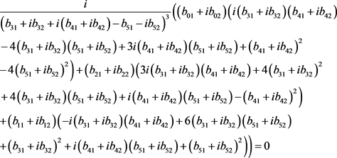 (14)
(14)
and
 (15)
(15)
Taking the real part and the imaginary parts of (14) and (15) and solving the corresponding equations with the help of an algebraic manipulator such as Mathematica we get the unique solution given in (5).
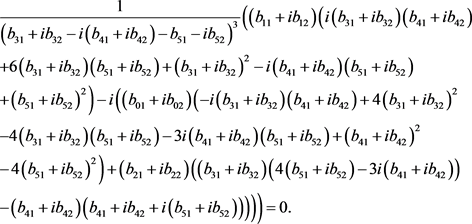
Now we assume that . In this case

Then

By condition (9) on v and since  for
for , we get
 (16)
(16)
and
 (17)
(17)
Taking the real part and the imaginary parts of (16) and (17) and solving the corresponding equations with the help of an algebraic manipulator such as Mathematica we get the unique solution given in (6).
Proof of Proposition 3. We will apply Theorem 5 to potential (7). Then its Darboux points are . Since

and consequently

Now applying condition (9) on v and taking into account that  for
for , we get

which yields

and

Therefore

Hence
![]()
This yields (8).
4. Conclusions
We have characterized the Liouville integrability of the Hamiltonian systems with Hamiltonian
![]()
and one of the following potentials
![]()
For doing this we have used the Darboux theory of integrability.
Acknowledgements
The first author is partially supported by the Ministerio de Economía, Industria y Competitividad, Agencia Estatal de Investigación grants MTM2016-77278-P (FEDER) and MDM-2014-0445, the Agència de Gestió d’Ajuts Universitaris i de Recerca grant 2017SGR1617, and the H2020 European Research Council grant MSCA-RISE-2017-777911. The second author is partially supported by FCT/Portugal through UID/MAT/ 04459/2013.