Two New Integrable Hierarchies and Their Nonlinear Integrable Couplings

Hui Chang, Yuxia Li^*

College of Electrical Engineering and Automation, Shandong University of Science and Technology, Qingdao, China.

DOI: 10.4236/jamp.2018.66113                

Abstract

By introducing an invertible linear transform, a new Lie algebra G is obtained from the Lie algebra H. Making use of the compatibility conditions of the respective isospectral problems, a generalized NLS-MKdV hierarchy and a new integrable soliton hierarchy are achieved by using the trace identity or the variational identity. Then, two special non-semisimple Lie algebras  and  are explicitly conducted. As an application, the nonlinear continuous integrable couplings of the obtained integrable systems as well as their bi-Hamiltonian structures are established, respectively.

Keywords

Non-Semisimple Lie algebra, Nonlinear Integrable Coupling, Hamiltonian Structure, Trace Identity, Variational Identity

1. Introduction

Integrable equations are a significant research topic of classical integrable systems. Thereinto, integrable coupling, as an extension of the integrable equation, was formulated and initialized with the clarity of the inner relationship between Virasoro algebras and hereditary operators [1] [2] . A few methods were presented by using perturbations [1] [2] , enlarging spectral problems [3] [4] [5] , creating higher-dimensional loop algebras [6] [7] , constructing a new algebraic system [8] [9] [10] , and making use of semi-direct sums of specific Lie algebras, for instance, the orthogonal Lie algebra $so\left(\mathrm{3,}R\right)$ , to construct some soliton hierarchies and their integrable couplings [11] - [16] . Much richer mathematical structures behind integrable couplings were explored, such as Lax pairs with several spectral parameters [17] [18] [19] , integrable constrained flows with higher multiplicity [20] [21] , local bi-Hamiltonian structures in higher dimensions and hereditary recursion operators of higher order [22] [23] . A lot of complex physical phenomena can be explained by all kinds of coupling systems [24] . Therefore, integrable couplings have attracted more and more attention from researchers in engineering and mathematical theory.

Thereinto, the nonlinear integrable couplings are a charming subject, which can be achieved by using an extended Lie algebra. First, an isospectral problem

${\varphi }_x=U\varphi ,U=U\left(u\right)=e_0+u_1{e}_1+u_2{e}_2+\cdots +u_s{e}_s,e_i,\varphi \in \tilde{A},$ (1)

and its auxiliary condition

${\varphi }_t=V\left(u\right)\varphi ,V=V\left(u\right)\in \tilde{A},$ (2)

admit a zero curvature equation

$U_t=V_x-\left[U,V\right],$ (3)

i.e., a Lax integrable system

$u_t=K\left(u\right),$ (4)

where $u={\left(u_1\mathrm{,}{u}_2\mathrm{,}\cdots \mathrm{,}{u}_s\right)}^{\text{T}}$ , $\tilde{A}$ is the corresponding loop algebra of a Lie algebra A. Next, take enlarged spectral matrices

$\bar{U}=\left(\begin{array}{cc}U& U_c\\ 0& U+U_c\end{array}\right)\text{and}\bar{V}=\left(\begin{array}{cc}V& V_c\\ 0& V+V_c\end{array}\right),$ (5)

in which $\bar{U}$ and $\bar{V}$ derive from (1) and (2), respectively, where $U_c=U_c\left(v\right)\in \tilde{A},\mathrm{<mi>\; </mi>}{V}_c=V_c\left(v\right)\in \tilde{A}$ , $v={\left(v_1\mathrm{,}{v}_2\mathrm{,}\cdots \mathrm{,}{v}_p\right)}^{\text{T}}$ and $\bar{u}$ consist of u and v. Then an enlarged zero curvature equation

${\bar{U}}_t={\bar{V}}_x-\left[\bar{U},\bar{V}\right],$ (6)

i.e.,

$\{\begin{array}{l}{U}_t=V_x-\left[U,V\right],\\ U_{c,t}=V_{c,x}-\left[U_c,V\right]-\left[U,V_c\right]-\left[U_c,V_c\right],\end{array}$ (7)

is a nonlinear integrable coupling of (3), because the commutator $\left[U_c\mathrm{,}{V}_c\right]$ can generate nonlinear terms.

In this paper, a new four-dimensional Lie algebra H is firstly presented, and another one G is obtained through an invertible linear transformation. A generalized NLS-MKdV hierarchy and a new integrable soliton hierarchy are achieved by using the Loop algebras $\tilde{H}$ and $\tilde{G}$ of H and G in Section 2. Two special non-semisimple Lie algebras $\bar{H}$ and $\bar{G}$ are determined programmatically, and its associated nonlinear continuous integrable couplings and their bi-Hamiltonian structures are established in Section 3. Finally, concluding remarks are given, as well as some proposals for the future work.

2. Two New Hamiltonian Hierarchies

2.1. Two Lie Algebras

A Lie algebra $H=\text{span}{\left\{h_i\right\}}_{i=1}^4$ is presented

$h_1=\left(\begin{array}{ccc}1& 0& -1\\ 0& -2& 0\\ -1& 0& 1\end{array}\right),h_2=\left(\begin{array}{ccc}1& 0& 1\\ 0& -2& 0\\ 1& 0& 1\end{array}\right),h_3=\left(\begin{array}{ccc}0& 1& 0\\ 1& 0& -1\\ 0& -1& 0\end{array}\right),h_4=\left(\begin{array}{ccc}0& 1& 0\\ -1& 0& 1\\ 0& -1& 0\end{array}\right),$ (8)

with

$\begin{array}{l}\left[h_1,h_2\right]=0,\left[h_1,h_3\right]=4h_4,\left[h_1,g_h\right]=4h_3,\\ \left[h_2,h_3\right]=2h_4,\left[h_2,h_4\right]=2h_3,\left[h_3,h_4\right]=-2h_1.\end{array}$ (9)

An invertible linear transformation can be established as follows:

$L:H\to G,g_i={\displaystyle \underset{i=1}{\overset{4}{\sum }}}B{h}_i\text{and}B={\left(b_{ij}\right)}_{4\times 4},\det \left(B\right)\ne 0,$ (10)

Specially, taking

$B=\left(\begin{array}{cccc}1& 0& 0& 0\\ \frac{1}{2}& -\frac{1}{2}& 0& 0\\ 0& 0& \frac{1}{2}& \frac{1}{2}\\ 0& 0& \frac{1}{2}& -\frac{1}{2}\end{array}\right),{\left(g_1,g_2,g_3,g_4\right)}^{\text{T}}=B{\left(h_1,h_2,h_3,h_4\right)}^{\text{T}},$ (11)

results in a new Lie algebra $G=\text{span}{\left\{g_i\right\}}_{i=1}^4$ , where

$g_1=\left(\begin{array}{ccc}1& 0& -1\\ 0& -2& 0\\ -1& 0& 1\end{array}\right),g_2=\left(\begin{array}{ccc}0& 0& -1\\ 0& 0& 0\\ -1& 0& 0\end{array}\right),g_3=\left(\begin{array}{ccc}0& 1& 0\\ 0& 0& 0\\ 0& -1& 0\end{array}\right),g_4=\left(\begin{array}{ccc}0& 0& 0\\ 1& 0& -1\\ 0& 0& 0\end{array}\right),$ (12)

equipped with

$\begin{array}{l}\left[g_1,g_2\right]=0,\left[g_1,g_3\right]=4g_3,\left[g_1,g_4\right]=-4g_4,\\ \left[g_2,g_3\right]=g_3,\left[g_2,g_4\right]=-g_4,\left[g_3,g_4\right]=g_1.\end{array}$ (13)

In what follows, the corresponding loop algebras $\tilde{H}$ and $\tilde{G}$ of the Lie algebras H and G are introduced, respectively. Let $\tilde{H}=\left\{h|h\in \mathcal{C}\left[\lambda \right]\otimes H\right\}$ , $\tilde{G}=\left\{g\mathrm{<mo>\; |\; </mo>}g\in \mathcal{C}\left[\lambda \right]\otimes G\right\}$ , where a loop algebra $\mathcal{C}\left[\lambda \right]\otimes H$ is defined by $\text{span}\left\{{\lambda }^{kn+i}h\mathrm{<mo>\; |\; </mo>}n\in \mathcal{Z}\mathrm{,}k\mathrm{,}i\in \mathcal{N}\mathrm{,}h\in H\right\}$ and $\mathcal{C}\left[\lambda \right]\otimes G$ is homoplastically defined by $\text{span}\left\{{\lambda }^{kn+i}g\mathrm{<mo>\; |\; </mo>}n\in \mathcal{Z}\mathrm{,}k\mathrm{,}i\in \mathcal{N}\mathrm{,}h\in H\right\}$ , $\mathcal{C}\left[\lambda \right]$ represents a set of Laurent polynomials in $\lambda$ . Taking $h_j\left(n,i\right)=h_j{\lambda }^{kn+i},j=1,2,3,4$ , the commutator relations of $\tilde{H}$ are

$\{\begin{array}{l}\left[h_1\left(m,i\right),h_2\left(n,j\right)\right]=0,\left[h_1\left(m,i\right),h_3\left(n,j\right)\right]=4h_4\left({\epsilon }_{i,j},{\delta }_{i,j}\right),\hfill \\ \left[h_1\left(m,i\right),h_4\left(n,j\right)\right]=4h_3\left({\epsilon }_{i,j},{\delta }_{i,j}\right),\left[h_2\left(m,i\right),h_3\left(n,j\right)\right]=2h_4\left({\epsilon }_{i,j},{\delta }_{i,j}\right),\hfill \\ \left[h_2\left(m,i\right),h_4\left(n,j\right)\right]=2h_3\left({\epsilon }_{i,j},{\delta }_{i,j}\right),\left[h_3\left(m,i\right),h_4\left(n,j\right)\right]=-2h_1\left({\epsilon }_{i,j},{\delta }_{i,j}\right),\hfill \\ {\epsilon }_{i,j}=\{\begin{array}{l}m+n,i+j<k,\hfill \\ m+n+1,i+j>k,\hfill \end{array}{\delta }_{i,j}=\{\begin{array}{l}i+j,i+j<k,\hfill \\ i+j-k,i+j>k.\hfill \end{array}\hfill \end{array}$ (14)

Similarly, the commutator relations of the loop algebra $\tilde{G}$ have

$\{\begin{array}{l}\left[g_1\left(m,i\right),g_2\left(n,j\right)\right]=0,\left[g_1\left(m,i\right),g_3\left(n,j\right)\right]=4g_3\left({\epsilon }_{i,j},{\delta }_{i,j}\right),\hfill \\ \left[g_1\left(m,i\right),g_4\left(n,j\right)\right]=-4g_4\left({\epsilon }_{i,j},{\delta }_{i,j}\right),\left[g_2\left(m,i\right),g_3\left(n,j\right)\right]=g_3\left({\epsilon }_{i,j},{\delta }_{i,j}\right),\hfill \\ \left[g_2\left(m,i\right),g_4\left(n,j\right)\right]=-g_4\left({\epsilon }_{i,j},{\delta }_{i,j}\right),\left[g_3\left(m,i\right),g_4\left(n,j\right)\right]=g_1\left({\epsilon }_{i,j},{\delta }_{i,j}\right),\hfill \\ {\epsilon }_{i,j}=\{\begin{array}{l}m+n,i+j<k,\hfill \\ m+n+1,i+j>k\hfill \end{array}{\delta }_{i,j}=\{\begin{array}{l}i+j,i+j<k,\hfill \\ i+j-k,i+j>k.\hfill \end{array}\hfill \end{array}$ (15)

Note that the commutator operations in loop algebras $\tilde{G}$ and $\tilde{W}$ are closed. In the following section, one endeavor to deduce two soliton hierarchies by using the two Lie algebras.

2.2. Two New Integrable Hierarchies

2.2.1. Generalized NLS-MKdV Hierarchy

Let $k=1,i=0$ , $\tilde{H}$ is reduced to the simplest loop algebra

$\widetilde{H_1}=span{\left\{h_j\left(n\right)\right\}}_{j=1}^4$

where $h_j\left(n\right)=h_j{\lambda }^n$ . Considering the spectral matrix

${\phi }_x=U\phi ,U=h_2\left(1\right)+q{h}_1\left(0\right)+r{h}_3\left(0\right)+s{h}_4\left(0\right),$ (16)

and setting

$W={\displaystyle \underset{m\ge 0}{\sum }}\left(a_m{h}_1\left(-m\right)+b_m{h}_3\left(-m\right)+c_m{h}_4\left(-m\right)\right),$ (17)

the stationary zero curvature equation

$W_x=\left[U,W\right],$ (18)

admits the recurrence relations for W as follows:

$\{\begin{array}{l}{a}_{mx}=-2r{c}_m+2s{b}_m,\\ b_{mx}=2c_{m+1}+4q{c}_m-4s{a}_m,\\ c_{mx}=2b_{m+1}+4q{b}_m-4r{a}_m.\end{array}$ (19)

Note that

$\begin{array}{l}{V}_{+}^{\left(n\right)}={\left({\lambda }^{n}W\right)}_{+}={\displaystyle \underset{m=0}{\overset{n}{\sum }}}\left(a_m{h}_1\left(n-m\right)+b_m{h}_3\left(n-m\right)+c_m{h}_4\left(n-m\right)\right),\\ V_{-}^{\left(n\right)}={\lambda }^{n}W-V_{+}^{\left(n\right)}.\end{array}$

Then (18) can be reset below:

$-V_{+x}^{\left(n\right)}+\left[U,V_{+}^{\left(n\right)}\right]=V_{-x}^{\left(n\right)}-\left[U,V_{-}^{\left(n\right)}\right].$ (20)

A direct calculation has $-V_{+x}^{\left(n\right)}+\left[U,V_{+}^{\left(n\right)}\right]=2c_{n+1}{h}_3\left(0\right)+2b_{n+1}{h}_4\left(0\right)$ . Taking $V^{\left(n\right)}=V_{+}^{\left(n\right)}+{\Delta }_n,\mathrm{<mi>\; </mi>}{\Delta }_n=a_{n+1}{h}_1\left(0\right)$ , the zero curvature equation

$U_t=V_x^{\left(n\right)}-\left[U,V^{\left(n\right)}\right],$ (21)

leads to the following integrable hierarchy

$\{\begin{array}{l}{r}_x=-2c_{n+1}+4s{a}_{n+1},\\ s_x=-2b_{n+1}+4r{a}_{n+1},\\ q_x=a_{n+1x},\end{array}$ (22)

that is

$u_t={\left(\begin{array}{c}r\\ s\\ q\end{array}\right)}_t=J\left(\begin{array}{c}{b}_{n+1}\\ -c_{n+1}\\ 2a_{n+1}\end{array}\right)=JL\left(\begin{array}{c}{b}_n\\ -c_n\\ 2a_n\end{array}\right),J=\left(\begin{array}{ccc}0& 2& 2s\\ -2& 0& 2r\\ -2s& -2r& 0\end{array}\right),$ (23)

where

$L=\left(\begin{array}{ccc}-2q+4r{\partial }^{-1}s& -\frac{\partial }{2}+4r{\partial }^{-1}r& 0\\ -\frac{\partial }{2}-4s{\partial }^{-1}s& -2q-4s{\partial }^{-1}r& 0\\ -\frac{1}{2}{\partial }^{-1}r\partial -8{\partial }^{-1}sq& 2{\partial }^{-1}s\partial -8{\partial }^{-1}rq& 0\end{array}\right)=\left(\begin{array}{ccc}-2q& \frac{\partial }{2}& r\\ -\frac{\partial }{2}& -2q& -s\\ l_{31}& l_{32}& 0\end{array}\right),$ (24)

$\text{and}{l}_{31}=-\frac{1}{2}{\partial }^{-1}r\partial -8{\partial }^{-1}sq,l_{32}=2{\partial }^{-1}s\partial -8{\partial }^{-1}rq.$

Taking $q=0$ and the modified term ${\Delta }_n=0$ , the system (23) reduces to the NLS-MKTV hierarchy [25] . Therefore, (23) is named a generalized NLS-MKdV hierarchy.

2.2.2. A New Integrable Hierarchy

Letting $k=1,i=0$ of $\tilde{G}$ results in a loop algebra $\widetilde{G_1}=\text{span}{\left\{g_j\left(n\right)\right\}}_{j=1}^4$ , $deg\left(g_j\left(n\right)\right)=n$ , $n\in N$ . Considering the following spectral

${\phi }_{1x}=U_1{\phi }_1,U_1=g_2\left(1\right)+q_1{g}_1\left(0\right)+r_1{g}_3\left(0\right)+s_1{g}_4\left(0\right),$ (25)

and setting

$W_1={\displaystyle \underset{m\ge 0}{\sum }}\left(a_m{g}_1\left(-m\right)+b_m{g}_3\left(-m\right)+c_m{g}_4\left(-m\right)\right),$ (26)

the stationary zero curvature $W_{1x}=\left[U_1,W_1\right]$ admits the recurrence relations

$\{\begin{array}{l}{a}_{mx}=r_1{c}_m-s_1{b}_m,\hfill \\ b_{mx}=b_{m+1}+4q_1{b}_m-4r_1{a}_m,\hfill \\ c_{mx}=-c_{m+1}-4q_1{c}_m+4s_1{a}_m.\hfill \end{array}$ (27)

Note that $V_{1+}^{\left(n\right)}={\left({\lambda }^n{W}_1\right)}_{+}={\displaystyle \underset{m=0}{\overset{n}{\sum }}}\left(a_m{g}_1\left(n-m\right)+b_m{g}_3\left(n-m\right)+c_m{g}_4\left(n-m\right)\right)$ , and taking $V_1^{\left(n\right)}={\left({\lambda }^n{W}_1\right)}_{+}+{\Delta }_{n1},\mathrm{<mi>\; </mi>}{\Delta }_{n1}=a_{n+1}{g}_1\left(0\right)$ , the zero curvature equation $U_{1t}=V_{1x}^{\left(n\right)}-\left[U_1,V_1^{\left(n\right)}\right]$ leads to the integrable hierarchy

$u_{1t}={\left(\begin{array}{c}{r}_1\\ s_1\\ q_1\end{array}\right)}_t=\left(\begin{array}{c}-2c_{n+1}+4s_1{a}_{n+1}\\ -2b_{n+1}+4r_1{a}_{n+1}\\ a_{n+1x}\end{array}\right)=J_1\left(\begin{array}{c}{c}_{n+1}\\ b_{n+1}\\ 4a_{n+1}\end{array}\right)=J_1{L}_1\left(\begin{array}{c}{c}_n\\ b_n\\ 4a_n\end{array}\right),$ (28)

where

$J_1=\left(\begin{array}{ccc}0& -1& r_1\\ 1& 0& -s_1\\ -r_1& s_1& \frac{\partial }{2}\end{array}\right),L_1=\left(\begin{array}{ccc}-\partial -2q_1& 0& s_1\\ 0& \partial -2q_1& r_1\\ -4{\partial }^{-1}{r}_1\partial +16{\partial }^{-1}{r}_1{q}_1& -4{\partial }^{-1}{s}_1\partial +16{\partial }^{-1}{s}_1{q}_1& 8{\partial }^{-1}{r}_1{s}_1\end{array}\right).$(29)

2.3. Bi-Hamiltonian Structures of (23) and (28)

In this section, the bi-Hamiltonian structures of soliton hierarchies (23) and (28) are established. Firstly, the bi-Hamiltonian structure of (23) is obtained by applying the trace identity.

Letting

$V=\left(\begin{array}{ccc}a& b+c& -a\\ b-c& -2a& -b+c\\ -a& -b-c& a\end{array}\right),\mathrm{<mi>\; </mi>}a={\displaystyle \underset{n\ge 0}{\sum }}{a}_n{\lambda }^n,\mathrm{<mi>\; </mi>}b={\displaystyle \underset{n\ge 0}{\sum }}{b}_n{\lambda }^n,\mathrm{<mi>\; </mi>}c={\displaystyle \underset{n\ge 0}{\sum }}{c}_n{\lambda }^n,$ (30)

the bilinear forms $\langle V,U_{\lambda }\rangle =4a$ , $\langle V,U_r\rangle =4b$ , $\langle V,U_s\rangle =-4c$ , $\langle V,U_q\rangle =8a$ can be obtained by the calculation of $\langle A\mathrm{,}B\rangle =\text{tr}\left(AB\right)$ (A and B are square matrices). Substituting these results into the trace identity

$\left(\partial /\partial u_i\right)\langle V,U_{\lambda }\rangle =\left({\lambda }^{-\gamma }\left(\partial /\partial \lambda \right){\lambda }^{\gamma }\right)\langle V,U_{u_i}\rangle$ results in

$\frac{\delta }{\delta u}\left(4a\right)={\lambda }^{-\gamma }\frac{\partial }{\partial \lambda }{\lambda }^{\gamma }{\left(\begin{array}{c}4b\mathrm{,}-4c\mathrm{,8}a\end{array}\right)}^{\text{T}}\mathrm{.}$ (31)

Comparing of the coefficients of ${\lambda }^{-n-1}$ these both sides of the above equations, one has

$\frac{\delta }{\delta u}\left(a_{n+1}\right)={\lambda }^{-\gamma }\frac{\partial }{\partial \lambda }{\lambda }^{\gamma }{\left(\begin{array}{c}{b}_n\mathrm{,}-c_n\mathrm{,2}{a}_n\end{array}\right)}^{\text{T}}\mathrm{.}$ (32)

To fix the $\gamma$ , taking $n=1$ into (32) results in $\gamma =0$ . Therefore, the bi-Hamiltonian structure of (23) can be obtained below:

$u_t={\left(\begin{array}{c}r,s,q\end{array}\right)}_t^{\text{T}}=J\frac{\delta H_{n+1}}{\delta u}=JL\frac{\delta H_n}{\delta u}\text{where},H_{n+1}=\frac{a_{n+2}}{n+1}.$ (33)

It is easy to prove $JL=L^{*}J$ . Therefore, the hierarchy (33) is integrable in the Liouville sense.

Next, the bi-Hamiltonian structure of (28) is derived by using the trace identity. Letting

$V_1=\left(\begin{array}{ccc}a& b& -a\\ c& -2a& -c\\ -a& -b& a\end{array}\right),a={\displaystyle \underset{n\ge 0}{\sum }}{a}_n{\lambda }^n,b={\displaystyle \underset{n\ge 0}{\sum }}{b}_n{\lambda }^n,c={\displaystyle \underset{n\ge 0}{\sum }}{c}_n{\lambda }^n,$ (34)

the bilinear forms $\langle V_1,U_{1\lambda }\rangle =2a$ , $\langle V_1,U_{1r}\rangle =2c$ , $\langle V_1,U_{1s}\rangle =2b$ , $\langle V_1,U_{1q}\rangle =8a$ are computed, and $\frac{\delta }{\delta u}\left(2a\right)={\lambda }^{-\gamma }\frac{\partial }{\partial \lambda }{\lambda }^{\gamma }{\left(\begin{array}{c}2c\mathrm{,2}b\mathrm{,8}a\end{array}\right)}^{\text{T}}$ can be obtained similarly.

Comparing the coefficients of ${\lambda }^{-n-1}$ in the both side of the above equation yields

$\frac{\delta }{\delta u}\left(a_{n+1}\right)={\lambda }^{-\gamma }\frac{\partial }{\partial \lambda }{\lambda }^{\gamma }{\left(\begin{array}{c}{c}_n\mathrm{,}{b}_n\mathrm{,4}{a}_n\end{array}\right)}^{\text{T}}\mathrm{.}$ (35)

To fix the $\gamma$ , substituting $n=1$ into (35) results in $\gamma =0$ . Therefore, the bi-Hamiltonian structure of (28) can be established as follows:

$u_t={\left(\begin{array}{c}{r}_1,s_1,q_1\end{array}\right)}_t^{\text{T}}=J_1\frac{\delta H_{n+1}}{\delta u}=J_1{L}_1\frac{\delta H_n}{\delta u},\text{where},\mathrm{<mi>\; </mi>}{H}_{n+1}=\frac{a_{n+2}}{n+1}.$ (36)

It is easy to prove $J_1{L}_1=L_1^{*}{J}_1$ . Therefore, the hierarchy (36) is integrable in the Liouville sense.

3. Nonlinear Integrable Couplings of Soliton Hierarchies

3.1. Extension of Lie Algebras

Letting $\bar{H}=\text{span}{\left\{{\bar{h}}_i\right\}}_{i=1}^6$ , it is an extension of the Lie algebra H, where

$\begin{array}{l}{\bar{h}}_1=\left(\begin{array}{cc}{h}_1& \mathrm{<mi>\; </mi>0}\\ 0& \mathrm{<mi>\; </mi>}{h}_1\end{array}\right),{\bar{h}}_2=\left(\begin{array}{cc}{h}_2& \mathrm{<mi>\; </mi>0}\\ 0& \mathrm{<mi>\; </mi>}{h}_2\end{array}\right),{\bar{h}}_3=\left(\begin{array}{cc}{h}_3& \mathrm{<mi>\; </mi>0}\\ 0& \mathrm{<mi>\; </mi>}{h}_3\end{array}\right),{\bar{h}}_4=\left(\begin{array}{cc}{h}_4& \mathrm{<mi>\; </mi>0}\\ 0& \mathrm{<mi>\; </mi>}{h}_4\end{array}\right),\\ {\bar{h}}_5=\left(\begin{array}{cc}\mathrm{<mi>\; </mi>0}& \mathrm{<mi>\; </mi>}{h}_1\\ \mathrm{<mi>\; </mi>0}& \mathrm{<mi>\; </mi>}{h}_1\end{array}\right),{\bar{h}}_6=\left(\begin{array}{cc}\mathrm{<mi>\; </mi>0}& \mathrm{<mi>\; </mi>}{h}_2\\ \mathrm{<mi>\; </mi>0}& \mathrm{<mi>\; </mi>}{h}_2\end{array}\right),{\bar{h}}_7=\left(\begin{array}{cc}\mathrm{<mi>\; </mi>0}& \mathrm{<mi>\; </mi>}{h}_3\\ \mathrm{<mi>\; </mi>0}& \mathrm{<mi>\; </mi>}{h}_3\end{array}\right),{\bar{h}}_8=\left(\begin{array}{cc}\mathrm{<mi>\; </mi>0}& \mathrm{<mi>\; </mi>}{h}_4\\ \mathrm{<mi>\; </mi>0}& \mathrm{<mi>\; </mi>}{h}_4\end{array}\right).\end{array}$ (37)

Taking ${\bar{H}}_1=\text{span}\left\{{\bar{h}}_1\mathrm{,}{\bar{h}}_2\mathrm{,}{\bar{h}}_3\mathrm{,}{\bar{h}}_4\right\}$ , ${\bar{H}}_2=\text{span}\left\{{\bar{h}}_5\mathrm{,}{\bar{h}}_6\mathrm{,}{\bar{h}}_7\mathrm{,}{\bar{h}}_8\right\}$ yields

$\bar{H}={\bar{H}}_1\oplus {\bar{H}}_2,{\bar{H}}_1\cong {\bar{H}}_2\cong H,\left[{\bar{H}}_1,{\bar{H}}_2\right]\subseteq {\bar{H}}_2,$ (38)

which is a critical factor for generating nonlinear integrable couplings of integrable hierarchies. In order to seek a nonlinear integrable coupling of (23), a loop algebra of the Lie algebra $\bar{H}$ reads

$\widetilde{\stackrel{¯}{H}}=\text{span}\left\{{\bar{h}}_i\left(n\right)|{\bar{h}}_i\left(n\right)={\lambda }^n{\bar{h}}_i,n\in \mathcal{Z},{\bar{h}}_i\in \bar{H},i=1,2,3,4,5,6,7,8\right\}$

Similarly, letting $\bar{G}=\text{span}{\left\{{\bar{g}}_i\right\}}_{i=1}^6$ , where

$\begin{array}{l}{\bar{g}}_1=\left(\begin{array}{cc}{g}_1& \mathrm{<mi>\; </mi>0}\\ 0& \mathrm{<mi>\; </mi>}{g}_1\end{array}\right),{\bar{g}}_2=\left(\begin{array}{cc}{g}_2& \mathrm{<mi>\; </mi>0}\\ 0& \mathrm{<mi>\; </mi>}{g}_2\end{array}\right),{\bar{g}}_3=\left(\begin{array}{cc}{g}_3& \mathrm{<mi>\; </mi>0}\\ 0& \mathrm{<mi>\; </mi>}{g}_3\end{array}\right),{\bar{g}}_4=\left(\begin{array}{cc}{g}_4& \mathrm{<mi>\; </mi>0}\\ 0& \mathrm{<mi>\; </mi>}{g}_4\end{array}\right),\\ {\bar{g}}_5=\left(\begin{array}{cc}\mathrm{<mi>\; </mi>0}& \mathrm{<mi>\; </mi>}{g}_1\\ \mathrm{<mi>\; </mi>0}& \mathrm{<mi>\; </mi>}{g}_1\end{array}\right),{\bar{g}}_6=\left(\begin{array}{cc}\mathrm{<mi>\; </mi>0}& \mathrm{<mi>\; </mi>}{g}_2\\ \mathrm{<mi>\; </mi>0}& \mathrm{<mi>\; </mi>}{g}_2\end{array}\right),{\bar{g}}_7=\left(\begin{array}{cc}\mathrm{<mi>\; </mi>0}& \mathrm{<mi>\; </mi>}{g}_3\\ \mathrm{<mi>\; </mi>0}& \mathrm{<mi>\; </mi>}{g}_3\end{array}\right),{\bar{g}}_8=\left(\begin{array}{cc}\mathrm{<mi>\; </mi>0}& \mathrm{<mi>\; </mi>}{g}_4\\ \mathrm{<mi>\; </mi>0}& \mathrm{<mi>\; </mi>}{g}_4\end{array}\right).\end{array}$ (39)

Taking ${\bar{G}}_1=\text{span}\left\{{\bar{g}}_1\mathrm{,}{\bar{g}}_2\mathrm{,}{\bar{g}}_3\mathrm{,}{\bar{g}}_4\right\}$ , ${\bar{G}}_2=\text{span}\left\{{\bar{g}}_5\mathrm{,}{\bar{g}}_6\mathrm{,}{\bar{g}}_7\mathrm{,}{\bar{g}}_8\right\}$ results in

$\bar{G}={\bar{G}}_1\oplus {\bar{G}}_2,{\bar{G}}_1\cong {\bar{G}}_2\cong G,\left[{\bar{G}}_1,{\bar{G}}_2\right]\subseteq {\bar{G}}_2.$ (40)

And $\widetilde{\stackrel{¯}{G}}=\text{span}\left\{{\bar{g}}_i\left(n\right)|{\bar{g}}_i\left(n\right)={\lambda }^n{\bar{g}}_i,n\in \mathcal{Z},\bar{g}\in \bar{G},i=1,2,3,4,5,6,7,8\right\}$ is the corresponding loop algebra of $\bar{G}$ , which is enslaved to derive a integrable coupling of (28).

3.2. Nonlinear Continuous Integrable Couplings

3.2.1. Nonlinear Integrable Coupling of the Generalized NLS-MKdV Hierarchy

An enlarged spectral matrix associated with the loop algebra $\widetilde{\stackrel{¯}{H}}$ is introduced as follows:

${\bar{\phi }}_x=\bar{U}\bar{\phi },\bar{U}=\left(\begin{array}{cc}U& U_c\\ 0& U+U_c\end{array}\right),U_c=\left(\begin{array}{ccc}p& u+v& -p\\ u-v& -2p& -u+v\\ -p& -u-v& p\end{array}\right),$ (41)

i.e. $\bar{U}={\bar{h}}_2\left(1\right)+q{\bar{h}}_1\left(0\right)+r{\bar{h}}_3\left(0\right)+s{\bar{h}}_4\left(0\right)+p{\bar{h}}_5\left(0\right)+u{\bar{h}}_7\left(0\right)+v{\bar{h}}_8\left(0\right)$ , where U is defined by (16). Assume that

$\bar{W}={\displaystyle \underset{m\ge 0}{\sum }}\left(a_m{\bar{h}}_1\left(-m\right)+b_m{\bar{h}}_3\left(-m\right)+c_m{\bar{h}}_4\left(-m\right)+d_m{\bar{h}}_5\left(-m\right)+e_m{\bar{h}}_7\left(-m\right)+f_m{\bar{h}}_8\left(-m\right)\right),$

the stationary zero curvation ${\bar{W}}_x=\left[\bar{U},\bar{W}\right]$ admits the recurrence relations

$\{\begin{array}{l}{a}_{mx}=-2r{c}_m+2s{b}_m,\hfill \\ b_{mx}=2c_{m+1}+4q{c}_m-4s{a}_m,\hfill \\ c_{mx}=2b_{m+1}+4q{b}_m-4r{a}_m,\hfill \\ d_{mx}=-2\left(r+u\right)f_m+2v{b}_m-2u{c}_m+2\left(s+v\right)e_m,\hfill \\ e_{mx}=2f_{m+1}-4\left(s+v\right)d_m+4\left(p+q\right)f_m+4p{c}_m-4v{a}_m,\hfill \\ f_{mx}=2_{m+1}-4\left(r+u\right)d_m+4\left(p+q\right)e_m+4p{b}_m-4u{a}_m.\hfill \end{array}$ (42)

Choosing the initial values as $a_0=\alpha =const\ne 0$ , $d_0=\beta =const\ne 0$ , $b_0=c_0=e_0=f_0=0$ , and presuming ${a_m|}_{\bar{u}=0}={b_m|}_{\bar{u}=0}={c_m|}_{\bar{u}=0}={d_m|}_{\bar{u}=0}={e_m|}_{\bar{u}=0}=$ ${f_m|}_{\bar{u}=0}=0,$ (42) uniquely yields all differential polynomial functions $a_m\mathrm{,}{b}_m\mathrm{,}{c}_m\mathrm{,}{d}_m\mathrm{,}{e}_m$ and $f_m\mathrm{,}m\ge 0$ . The first few sets are

$\{\begin{array}{l}{b}_1=2\alpha r,c_1=2\alpha s,a_1=0;b_2=\alpha s_x-4\alpha qr,c_2=\alpha r_x-4\alpha qs,a_2=\alpha \left(s^2-r^2\right);\hfill \\ b_3=\frac{1}{2}\alpha r_{xx}-2\alpha {\left(qs\right)}_x-2\alpha q{s}_x+8\alpha q^{2}r+2\alpha r\left(s^2-r^2\right),\hfill \\ \begin{array}{l}{c}_3=\frac{1}{2}\alpha s_{xx}-2\alpha {\left(qr\right)}_x-2\alpha q{r}_x+8\alpha q^{2}s+2\alpha s\left(s^2-r^2\right),\\ a_3=\alpha \left(s{r}_x-r{s}_x\right)-4\alpha q\left(s^2-r^2\right);\end{array}\hfill \\ d_1=0,e_1=2\alpha u+2\beta \left(r+u\right),f_1=2\alpha v+2\beta \left(s+v\right);\hfill \\ e_2=\alpha v_x+\beta {\left(s+v\right)}_x-4\alpha u\left(p+q\right)-4\beta \left(r+u\right)\left(p+q\right)-4\alpha pr,\hfill \\ f_2=\alpha u_x+\beta {\left(r+u\right)}_x-4\alpha v\left(p+q\right)-4\beta \left(s+v\right)\left(p+q\right)-4\alpha ps,\hfill \\ d_2=2\alpha \left(sv-ru\right)+\alpha \left(v^2-u^2\right)+\beta {\left(s+v\right)}^2-\beta {\left(r+u\right)}^2;\hfill \\ \begin{array}{l}{e}_3=\alpha \left[\frac{1}{2}{u}_{xx}-8r{q}^2-2r\left(s^2-r^2\right)+4s_{x}q+2s{q}_x\right]+\frac{1}{2}\beta {\left(r+u\right)}_{xx}\\ -2\left(\alpha +\beta \right){\left[\left(s+v\right)\left(p+q\right)\right]}_x-2\left(\alpha +\beta \right){\left(s+v\right)}_x\left(p+q\right)\end{array}\hfill \\ +2\left(\alpha +\beta \right)\left(r+u\right)\left[4{\left(p+q\right)}^2-{\left(r+u\right)}^2+{\left(s+v\right)}^2\right],\hfill \\ \begin{array}{l}{f}_3=\alpha \left[\frac{1}{2}{v}_{xx}-8s{q}^2-2s\left(s^2-r^2\right)+4r_{x}q+2r{q}_x\right]+\frac{1}{2}\beta {\left(s+v\right)}_{xx}\\ -2\left(\alpha +\beta \right){\left[\left(r+u\right)\left(p+q\right)\right]}_x-2\left(\alpha +\beta \right){\left(r+u\right)}_x\left(p+q\right)\\ +2\left(\alpha +\beta \right)\left(s+v\right)\left[4{\left(p+q\right)}^2+{\left(s+v\right)}^2-{\left(r+u\right)}^2\right],\end{array}\hfill \\ d_3=\alpha \left(s{u}_x-s_{x}u+v{u}_x-v_{x}u+v{r}_x-v_{x}r\right)+\beta {\left(r+u\right)}_x\left(s+v\right)-\beta \left(r+u\right){\left(s+v\right)}_x\hfill \\ \mathrm{<mi>\; </mi>\; <mi>\; </mi>\; <mi>\; </mi>\; <mi>\; </mi>}+4\left(\alpha +\beta \right){\left(r+u\right)}^2\left(p+q\right)-4\left(\alpha +\beta \right){\left(s+v\right)}^2\left(p+q\right)+4\alpha q\left(s^2-r^2\right).\hfill \end{array}$(43)

Note that

$\begin{array}{l}{\bar{V}}_{+}^{\left(n\right)}={\left({\lambda }^n\bar{W}\right)}_{+}={\displaystyle \underset{m=0}{\overset{n}{\sum }}}(a_m{\bar{h}}_1\left(n-m\right)+b_m{\bar{h}}_3\left(n-m\right)+c_m{\bar{h}}_4\left(n-m\right)\\ +d_m{\bar{h}}_5\left(n-m\right)+e_m{\bar{h}}_7\left(n-m\right)+f_m{\bar{h}}_8\left(n-m\right)).\end{array}$ (44)

A direct calculation reads

$-{\bar{V}}_{+x}^{\left(n\right)}+\left[\bar{U},{\bar{V}}_{+}^{\left(n\right)}\right]=2c_{n+1}{\bar{h}}_3\left(0\right)+2b_{n+1}{\bar{h}}_4\left(0\right)+2e_{n+1}{\bar{h}}_7\left(0\right)+2b_{n+1}{\bar{h}}_8\left(0\right).$

Taking ${\bar{V}}^{\left(n\right)}={\bar{V}}_{+}^{\left(n\right)}+{\bar{\Delta }}_n,\mathrm{<mi>\; </mi>}{\bar{\Delta }}_n=a_{n+1}{\bar{h}}_1\left(0\right)+d_{n+1}{\bar{h}}_5\left(0\right)$ , the zero curvature equation

${\bar{U}}_t={\bar{V}}_x^{\left(n\right)}-\left[\bar{U},{\bar{V}}^{\left(n\right)}\right],$ (45)

leads to the following integrable hierarchy

${\bar{u}}_t={\left(\begin{array}{c}r\\ s\\ q\\ u\\ v\\ p\end{array}\right)}_t=\left(\begin{array}{c}-2c_{n+1}+4s{a}_{n+1}\\ -2b_{n+1}+4r{a}_{n+1}\\ a_{n+1x}\\ -2f_{n+1}+4r{a}_{n+1}+4s{d}_{n+1}+4v{d}_{n+1}\\ -2e_{n+1}+4u{a}_{n+1}+4r{d}_{n+1}+4u{d}_{n+1}\\ d_{n+1x}\end{array}\right).$ (46)

If $u=v=p=0$ , the system (46) is reduced to (23). According to the concept of nonlinear integrable couplings [26] [27] [28] , (46) is a nonlinear integrable coupling of (23).

3.2.2. Nonlinear Integrable Coupling of the Hierarchy (28)

An enlarged spectral matrix associated with the loop algebra $\widetilde{\stackrel{¯}{g}}$ is given below:

${\bar{\phi }}_x={\bar{U}}_1\bar{\phi },{\bar{U}}_1=\left(\begin{array}{cc}{U}_1& U_{1a}\\ 0& U_1+U_{1a}\end{array}\right),\mathrm{<mi>\; </mi>}{U}_{1a}=\left(\begin{array}{ccc}{p}_1& u_1& -p_1\\ -v_1& -2p_1& v_1\\ -p_1& -u_1& p_1\end{array}\right),$ (47)

that is,

${\bar{U}}_1={\bar{g}}_2\left(1\right)+q_1{\bar{g}}_1\left(0\right)+r_1{\bar{g}}_3\left(0\right)+s_1{\bar{g}}_4\left(0\right)+p_1{\bar{g}}_5\left(0\right)+u_1{\bar{g}}_7\left(0\right)+v_1{\bar{g}}_8(0)$

where $U_1$ is defined by (25). Assume that

$\begin{array}{c}{\bar{W}}_1={\displaystyle \underset{m\ge 0}{\sum }}(a_m{\bar{g}}_1\left(-m\right)+b_m{\bar{g}}_3\left(-m\right)+c_m{\bar{g}}_4\left(-m\right)\\ +d_m{\bar{g}}_5\left(-m\right)+e_m{\bar{g}}_7\left(-m\right)+f_m{\bar{g}}_8\left(-m\right)),\end{array}$

the stationary zero curvature equation ${\bar{W}}_{1x}=\left[{\bar{U}}_1,{\bar{W}}_1\right]$ admits the recurrence relations

$\{\begin{array}{l}{a}_{mx}=r_1{c}_m-s_1{b}_m,\hfill \\ b_{mx}=b_{m+1}+4q_1{b}_m-4r_1{a}_m,\hfill \\ c_{mx}=-c_{m+1}-4q_1{c}_m+4s_1{a}_m,\hfill \\ d_{mx}=\left(r_1+u_1\right)f_m-v_1{b}_m+u_1{c}_m-\left(s_1+v_1\right)e_m,\hfill \\ e_{mx}=e_{m+1}-4\left(r_1+u_1\right)d_m+4\left(p_1+q_1\right)e_m+4p_1{b}_m-4u_1{a}_m,\hfill \\ f_{mx}=-f_{m+1}-4\left(s_1+v_1\right)d_m-4\left(p_1+q_1\right)f_m-4p_1{c}_m+4v_1{a}_m.\hfill \end{array}$ (48)

Choosing the initial data as $a_0=\alpha =const\ne 0$ , $d_0=\beta =const\ne 0$ , $b_0=c_0=$ $e_0=f_0=0$ , and presuming ${a_m|}_{{\bar{u}}_1=0}={b_m|}_{{\bar{u}}_1=0}={c_m|}_{{\bar{u}}_1=0}={d_m|}_{{\bar{u}}_1=0}={e_m|}_{{\bar{u}}_1=0}={f_m|}_{{\bar{u}}_1=0}=0$ , the above-mentioned recursion relation uniquely engenders all differential polynomial functions $a_m\mathrm{,}{b}_m\mathrm{,}{c}_m\mathrm{,}{d}_m\mathrm{,}{e}_m$ and $f_m\mathrm{,}m\ge 0$ . The first few sets are listed as follows:

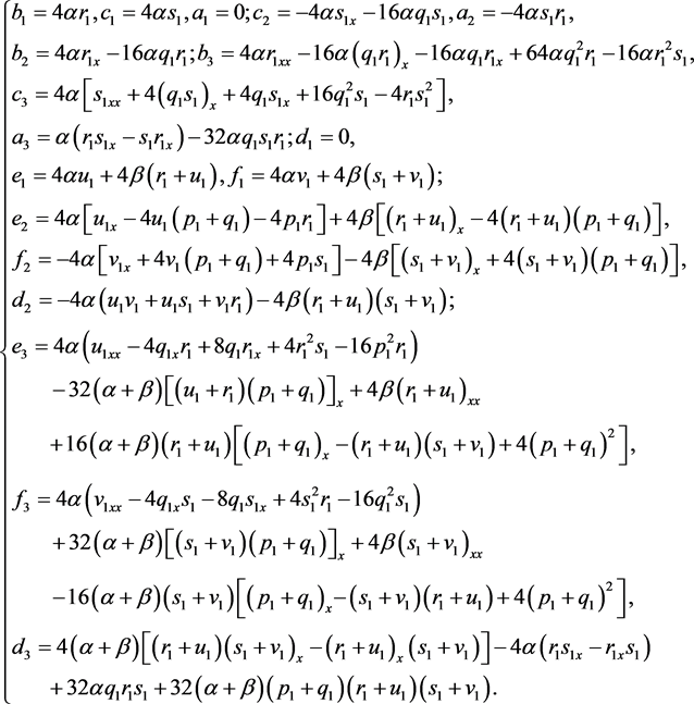
(49)

Note that

$\begin{array}{l}{\bar{V}}_{1+}^{\left(n\right)}={\left({\lambda }^n{\bar{W}}_1\right)}_{+}={\displaystyle \underset{m=0}{\overset{n}{\sum }}}(a_m{\bar{g}}_1\left(n-m\right)+b_m{\bar{g}}_3\left(n-m\right)+c_m{\bar{g}}_4\left(n-m\right)\\ +d_m{\bar{g}}_5\left(n-m\right)+e_m{\bar{g}}_7\left(n-m\right)+f_m{\bar{g}}_8\left(n-m\right)).\end{array}$ (50)

A direct calculation reads

$-{\bar{V}}_{1+x}^{\left(n\right)}+\left[{\bar{U}}_1,{\bar{V}}_{1+}^{\left(n\right)}\right]=-b_{n+1}{\bar{g}}_3\left(0\right)+c_{n+1}{\bar{g}}_4\left(0\right)-e_{n+1}{\bar{g}}_7\left(0\right)+f_{n+1}{\bar{g}}_8\left(0\right).$

Taking ${\bar{V}}_1^{\left(n\right)}={\bar{V}}_{1+}^{\left(n\right)}+{\bar{\Delta }}_{n1},{\bar{\Delta }}_{n1}=a_{n+1}{\bar{g}}_1\left(0\right)+d_{n+1}{\bar{g}}_5\left(0\right)$ , the zero curvature equation

${\bar{U}}_{1t}={\bar{V}}_{1x}^{\left(n\right)}-\left[{\bar{U}}_1\mathrm{,}{\bar{V}}_1^{\left(n\right)}\right]\mathrm{,}$ (51)

leads to the following integrable hierarchy

$u_{1t}={\left(\begin{array}{c}{r}_1\\ s_1\\ q_1\\ u_1\\ v_1\\ p_1\end{array}\right)}_t=\left(\begin{array}{c}-b_{n+1}+4r_1{a}_{n+1}\\ c_{n+1}+4s_1{a}_{n+1}\\ a_{n+1,x}\\ -e_{n+1}+4u_1{a}_{n+1}+4r_1{d}_{n+1}+4u_1{d}_{n+1}\\ f_{n+1}-4v_1{a}_{n+1}-4s_1{d}_{n+1}-4v_1{d}_{n+1}\\ d_{n+1,x}\end{array}\right).$ (52)

If $u_1=v_1=p_1=0$ , (52) is reduced to (28), and (52) is a nonlinear integrable coupling of (28).

3.3. Bi-Hamiltonian Structures of Nonlinear Integrable Couplings

3.3.1. Bilinear Forms

In this section, the bi-Hamiltonian structures of the nonlinear integrable couplings of the generalized NLS-MKdV hierarchy (23) and the new integrable hierarchy (28) can be established. In order to achieve this target, two non-degenerate, symmetric and ad-invariant bilinear forms on two Lie algebras $\bar{H}$ and $\bar{G}$ are introduced. First of all, an isomorphic mapping $\sigma$ between the Lie algebra $\bar{H}$ and a vector space R⁸ is established that

$\sigma :\bar{H}\to R^8,A\mapsto \left(a_1,a_2,\cdots ,a_8\right),A={\displaystyle \underset{i=1}{\overset{8}{\sum }}}{a}_i{\bar{h}}_i,$ (53)

which imports a Lie algebraic system on R⁸. The corresponding commutator $\left[\mathrm{.\; <mi>\; </mi>,.}\right]$ on R⁸ is given by

${\left[a,b\right]}_{1R^8}^{\text{T}}=\sigma {\left[A_1,B_1\right]}_{\bar{H}}=a^{\text{T}}{R}_1\left(b\right),$ (54)

where $a\mathrm{,}b\in R^8$ , $A_1\mathrm{,}{B}_1\in \bar{H}$ ,

$R_1\left(b\right)=\left(\begin{array}{cccccccc}0& 0& 4b_4& 4b_3& 0& 0& 4b_8& 4b_7\\ 0& 0& 2b_4& 2b_3& 0& 0& 2b_8& 2b_7\\ -2b_4& 0& 0& -4b_1-2b_2& -2b_8& 0& 0& -4b_5-2b_6\\ 2b_3& 0& -4b_1-2b_2& 0& 2b_7& 0& -4b_5-2b_6& 0\\ 0& 0& 0& 0& 0& 0& 4b_4+4b_8& 4b_3+4b_7\\ 0& 0& 0& 0& 0& 0& 2b_4+2b_8& 2b_3+2b_7\\ 0& 0& 0& 0& -2b_4-2b_8& 0& 0& b_{78}\\ 0& 0& 0& 0& 2b_3+2b_7& 0& b_{87}& 0\end{array}\right)$ (55)

is a square matrix and $b_{78}=-4b_1-2b_2-4b_5-2b_6$ , $b_{87}=-4b_1-2b_2-4b_5-2b_6$ . The bilinear form $\langle a\mathrm{,}b\rangle =a^{\text{T}}{F}_{1}b$ on R⁸ is determined. Simultaneously, $F_1^{\text{T}}=F_1$ and

${\left(R_1\left(b\right)F_1\right)}^{\text{T}}=-R_1\left(b\right)F_1\mathrm{,}\text{for}\text{all}\mathrm{<mi>\; </mi>}b\in R^8$ (56)

are ascertained in accordance with the symmetric property $\langle a\mathrm{,}b\rangle =\langle b\mathrm{,}a\rangle$ , and the ad-invariance property $\langle a\mathrm{,}\left[b\mathrm{,}c\right]\rangle =\langle \left[a\mathrm{,}b\right]\mathrm{,}c\rangle$ , where $F_1$ is an $8\times 8$ constant matrix. Solving the matrix Equation (56) yields

$F_1=\left(\begin{array}{cccccccc}2{\eta }_1\mathrm{<mi>\; </mi>}& {\eta }_1& 0& 0& 2{\eta }_2\mathrm{<mi>\; </mi>}& {\eta }_2& 0& 0\\ {\eta }_1& 0& 0& 0& {\eta }_2& 0& 0& 0\\ 0& 0& {\eta }_1& 0& 0& 0& {\eta }_2& 0\\ 0& 0& 0& -{\eta }_1& 0& 0& 0& -{\eta }_2\\ 2{\eta }_2\mathrm{<mi>\; </mi>}& {\eta }_2& 0& 0& 2{\eta }_2\mathrm{<mi>\; </mi>}& {\eta }_2& 0& 0\\ {\eta }_2& 0& 0& 0& {\eta }_2& 0& 0& 0\\ 0& 0& {\eta }_2& 0& 0& 0& {\eta }_2& 0\\ 0& 0& 0& -{\eta }_2& 0& 0& 0& -{\eta }_2\end{array}\right),$ (57)

where ${\eta }_1$ and ${\eta }_2$ are arbitrary constants, and $\left({\eta }_1-{\eta }_2\right){\eta }_2\ne 0$ . Thus, a bilinear form is defined on the Lie algebra $\bar{H}$ by

$\begin{array}{c}{\langle A_1,B_1\rangle }_{\bar{H}}={\langle {\sigma }^{-1}\left(A_1\right),{\sigma }^{-1}\left(B_1\right)\rangle }_{R^8}=a^{\text{T}}{F}_{1}b\\ ={\eta }_1\left[\left(2a_1+a_2\right)b_1+a_1{b}_2+a_3{b}_3-a_4{b}_4\right]+{\eta }_2(2a_5{b}_1\\ +a_6{b}_1+a_5{b}_2+a_7{b}_3-a_8{b}_4+\left(2a_1+a_2+2a_5+a_6\right)b_5\\ +\left(a_1+a_5\right)b_6+\left(a_3+a_7\right)b_7-\left(a_4+a_8\right)b_8).\end{array}$ (58)

Similarly, an isomorphic mapping $\rho$ is established between the Lie algebra $\bar{G}$ and a vector space R⁸:

$\rho :\bar{G}\to R^8,A\mapsto \left(a_1,a_2,\cdots ,a_8\right),A={\displaystyle \underset{i=1}{\overset{8}{\sum }}}{a}_i{\bar{g}}_i.$ (59)

The corresponding commutator $\left[\mathrm{.\; <mi>\; </mi>,.}\right]$ on R⁸ is given by

${\left[a,b\right]}_{2R^8}^{\text{T}}=\rho \left[A_2,B_2\right]=a^{\text{T}}{R}_2\left(b\right),$ (60)

where $a\mathrm{,}b\in R^8$ , $A_2\mathrm{,}{B}_2\in \bar{G}$ and $R_2\left(b\right)$ is a square matrix

$R_2\left(b\right)=\left(\begin{array}{cccccccc}0& 0& 4b_3& -4b_4& 0& 0& 4b_7& -4b_8\\ 0& 0& b_3& -b_4& 0& 0& b_7& -b_8\\ b_4& 0& -4b_1-b_2& 0& b_8& 0& -4b_5-b_6& 0\\ -b_3& 0& 0& 4b_1+b_2& -b_7& 0& 0& 4b_5+b_6\\ 0& 0& 0& 0& 0& 0& 4b_3+4b_7& -4b_4-4b_8\\ 0& 0& 0& 0& 0& 0& b_3+b_7& -b_4-b_8\\ 0& 0& 0& 0& b_4+b_8& 0& b_{77}& 0\\ 0& 0& 0& 0& -b_3-b_7& 0& 0& b_{88}\end{array}\right),$ (61)

and $b_{77}=-4b_1-b_2-4b_5-b_6,b_{88}=4b_1+b_2+4b_5+b_6$ . According to $F_2^{\text{T}}=F_2$ , solving the matrix equation ${\left(R_2\left(b\right)F_2\right)}^{\text{T}}=-R_2\left(b\right)F_2$ results in

$F_2=\left(\begin{array}{cccccccc}2{\zeta }_1& {\zeta }_1& 0& 0& 2{\zeta }_2& {\zeta }_2& 0& 0\\ {\zeta }_1& 0& 0& 0& {\zeta }_2& 0& 0& 0\\ 0& 0& 0& {\zeta }_1& 0& 0& 0& {\zeta }_2\\ 0& 0& {\zeta }_1& 0& 0& 0& {\zeta }_2& 0\\ 2{\zeta }_2& {\zeta }_2& 0& 0& 2{\zeta }_2& {\zeta }_2& 0& 0\\ {\zeta }_2& 0& 0& 0& {\zeta }_2& 0& 0& 0\\ 0& 0& 0& {\zeta }_2& 0& 0& 0& {\zeta }_2\\ 0& 0& {\zeta }_2& 0& 0& 0& {\zeta }_2& 0\end{array}\right),$ (62)

where ${\zeta }_1$ and ${\zeta }_2$ are arbitrary constants, and $\left({\zeta }_1-{\zeta }_2\right){\zeta }_2\ne 0$ . Therefore, a bilinear form

$\begin{array}{c}{\langle A_2,B_2\rangle }_{\bar{G}}={\langle {\rho }^{-1}\left(A_2\right),{\rho }^{-1}\left(B_2\right)\rangle }_{R^8}=a^{\text{T}}{F}_{2}b\\ ={\zeta }_1\left[\left(4a_1+a_2\right)b_1+a_1{b}_2+a_4{b}_3+a_3{b}_4\right]+{\zeta }_2(4a_5{b}_1\\ +a_6{b}_1+a_5{b}_2+a_8{b}_3+a_7{b}_4+\left(4a_1+a_2+4a_5+a_6\right)b_5\\ +\left(a_1+a_5\right)b_6+\left(a_4+a_8\right)b_7+\left(a_3+a_7\right)b_8)\end{array}$ (63)

is defined on the Lie algebra $\bar{G}$ , where $A_2={\displaystyle \underset{i=1}{\overset{8}{\sum }}}{a}_i{\bar{g}}_i,B_2={\displaystyle \underset{i=1}{\overset{8}{\sum }}}{b}_i{\bar{g}}_i,a,b\in \bar{G}$ .

Obviously, the bilinear forms (58) and (63) are non-degenerate, symmetric and ad-invariant associated with the Lie product.

3.3.2. Bi-Hamiltonian Structures of the Integrable Hierarchies (46) and (52)

Let

$\bar{V}=\left(\begin{array}{cc}V& V_a\\ 0& V+V_a\end{array}\right),d={\displaystyle \underset{n\ge 0}{\sum }}{d}_n{\lambda }^n,e={\displaystyle \underset{n\ge 0}{\sum }}{e}_n{\lambda }^n,f={\displaystyle \underset{n\ge 0}{\sum }}{f}_n{\lambda }^n,$ (64)

where $V_a=\left(\begin{array}{ccc}d& e+f& -d\\ e-f& -2d& -e+f\\ -d& -e-f& d\end{array}\right)$ , V is defined by (30). The bilinear forms

can be calculated according to (58), as follows:

$\begin{array}{l}\langle \bar{V},{\bar{U}}_{\lambda }\rangle ={\eta }_{1}a+{\eta }_{2}d,\langle \bar{V},{\bar{U}}_r\rangle ={\eta }_{1}b+{\eta }_{2}e,\langle \bar{V},{\bar{U}}_s\rangle =-{\eta }_{1}c-{\eta }_{2}f,\\ \langle \bar{V},{\bar{U}}_q\rangle =2{\eta }_{1}a+2{\eta }_{2}d,\langle \bar{V},{\bar{U}}_u\rangle ={\eta }_2\left(b+e\right),\\ \langle \bar{V},{\bar{U}}_v\rangle =-{\eta }_2\left(c+f\right),\langle \bar{V},{\bar{U}}_p\rangle =2{\eta }_2\left(a+d\right),\end{array}$ (65)

where $\bar{U}$ is defined by (41). Substituting (65) into the Variational identity [27] , and comparing the coefficients of ${\lambda }^{-n-1}$ yields

$\frac{\delta }{\delta \bar{u}}{\displaystyle \int }\left({\eta }_1{a}_{n+1}+{\eta }_2{d}_{n+1}\right)\text{d}x=\left(-n+\gamma \right)\left(\begin{array}{c}{\eta }_1{b}_n+{\eta }_2{e}_n\\ -\left({\eta }_1{c}_n+{\eta }_2{f}_n\right)\\ 2{\eta }_1{a}_n+2{\eta }_2{d}_n\\ {\eta }_2\left(b_n+e_n\right)\\ -{\eta }_2\left(c_n+f_n\right)\\ 2{\eta }_2\left(a_n+d_n\right)\end{array}\right).$ (66)

It is easy to see $\gamma =0$ . The adjoint symmetrical function of system (46) reads

$\left(\begin{array}{c}{\eta }_1{b}_n+{\eta }_2{e}_n\\ -\left({\eta }_1{c}_n+{\eta }_2{f}_n\right)\\ 2{\eta }_1{a}_n+2{\eta }_2{d}_n\\ {\eta }_2\left(b_n+e_n\right)\\ -{\eta }_2\left(c_n+f_n\right)\\ 2{\eta }_2\left(a_n+d_n\right)\end{array}\right)\equiv \frac{\delta H_n}{\delta \bar{u}}\mathrm{,\; <mi>\; </mi>}\text{where}\mathrm{<mi>\; </mi>}{H}_n=\frac{\delta }{\delta \bar{u}}{\displaystyle \int }\frac{-{\eta }_1{a}_{n+1}-{\eta }_2{d}_{n+1}}{n}\text{d}x\mathrm{.}$ (67)

Therefore, the bi-Hamiltonian structure of the nonlinear integrable coupling of the hierarchy (23) can be established as follows:

${\bar{u}}_t={\left(r,s,q,u,v,p\right)}_t^{\text{T}}=\bar{J}\frac{\delta H_{n+1}}{\delta \bar{u}}=\bar{J}\bar{L}\frac{\delta H_n}{\delta \bar{u}},$ (68)

where

$\bar{J}=\frac{1}{{\eta }_1-{\eta }_2}\left(\begin{array}{cc}J& -J\\ -J& J_c\end{array}\right),\bar{L}=\left(\begin{array}{cc}L& L_c\\ 0& L+L_c\end{array}\right),$ (69)

$\begin{array}{l}{J}_c=\left(\begin{array}{ccc}0& \frac{2{\eta }_1}{{\eta }_2}& 2s\frac{{\eta }_1}{{\eta }_2}+2v\frac{{\eta }_1-{\eta }_2}{{\eta }_2}\\ -\frac{2{\eta }_1}{{\eta }_2}& 0& 2r\frac{{\eta }_1}{{\eta }_2}+2u\frac{{\eta }_1-{\eta }_2}{{\eta }_2}\\ -2s\frac{{\eta }_1}{{\eta }_2}+2v\frac{{\eta }_2-{\eta }_1}{{\eta }_2}& -2r\frac{{\eta }_1}{{\eta }_2}+2u\frac{{\eta }_2-{\eta }_1}{{\eta }_2}& \frac{{\eta }_1}{{\eta }_2}\partial \end{array}\right),\\ L_{1c}=\left(\begin{array}{ccc}-2p& 0& u\\ 0& 2p& -2v\\ {\bar{l}}_{31}& {\bar{l}}_{32}& {\bar{l}}_{33}\end{array}\right),\end{array}$ (70)

${\bar{l}}_{31}=-2{\partial }^{-1}u\partial -8{\partial }^{-1}vq-8{\partial }^{-1}sp-18{\partial }^{-1}vp$ ,

${\bar{l}}_{32}=-2{\partial }^{-1}v\partial -8{\partial }^{-1}uq-8{\partial }^{-1}rp-8{\partial }^{-1}up$ , ${\bar{l}}_{33}=4{\partial }^{-1}vr-4{\partial }^{-1}sr$

J and L are defined in (23) and (24), respectively, and $\bar{J}$ is a Hamiltonian operator.

Similarly, let

${\bar{V}}_1=\left(\begin{array}{cc}{V}_1& V_{1a}\\ 0& V_1+V_{1a}\end{array}\right),d={\displaystyle \underset{n\ge 0}{\sum }}{d}_n{\lambda }^n,e={\displaystyle \underset{n\ge 0}{\sum }}{e}_n{\lambda }^n,f={\displaystyle \underset{n\ge 0}{\sum }}{f}_n{\lambda }^n,$ (71)

where $V_{1a}=\left(\begin{array}{ccc}d& e& -d\\ f& -2d& -f\\ -d& -e& d\end{array}\right)$ , $V_1$ is defined by (34). Then, the bilinear forms are computed according to (63), as follows:

$\begin{array}{l}\langle {\bar{V}}_1,{\bar{U}}_{1\lambda }\rangle ={\zeta }_{1}a+{\zeta }_{2}d,\langle \bar{V},{\bar{U}}_{1r}\rangle ={\zeta }_{1}c+{\zeta }_{2}c,\langle {\bar{V}}_1,{\bar{U}}_{1s}\rangle ={\zeta }_{1}b+{\zeta }_{2}e,\\ \langle {\bar{V}}_1,{\bar{U}}_{1q}\rangle =4{\zeta }_{1}a+4{\zeta }_{2}d,\langle {\bar{V}}_1,{\bar{U}}_{1u}\rangle ={\zeta }_2\left(c+f\right),\\ \langle {\bar{V}}_1,{\bar{U}}_{1v}\rangle =-{\zeta }_2\left(b+e\right),\langle {\bar{V}}_1,{\bar{U}}_{1p}\rangle =4{\zeta }_2\left(a+d\right),\end{array}$ (72)

where ${\bar{U}}_1$ is defined by (47). Substituting (72) into the Variational identity, and comparing the coefficients of ${\lambda }^{-n-1}$ yields

$\frac{\delta }{\delta \bar{u}}{\displaystyle \int }\left({\zeta }_1{a}_{n+1}+{\zeta }_2{d}_{n+1}\right)\text{d}x=\left(-n+\gamma \right)\left(\begin{array}{c}{\zeta }_1{c}_n+{\zeta }_2{f}_n\\ {\zeta }_1{b}_n+{\zeta }_2{e}_n\\ 4{\zeta }_1{a}_n+4{\zeta }_2{d}_n\\ {\zeta }_2\left(c_n+f_n\right)\\ {\zeta }_2\left(b_n+e_n\right)\\ 4{\zeta }_2\left(a_n+d_n\right)\end{array}\right)\mathrm{.}$ (73)

It is easy to see $\gamma =0$ , the adjoint symmetrical function of the integrable system (53) has

$\left(\begin{array}{c}{\zeta }_1{c}_n+{\zeta }_2{f}_n\\ {\zeta }_1{b}_n+{\zeta }_2{e}_n\\ 4{\zeta }_1{a}_n+4{\zeta }_2{d}_n\\ {\zeta }_2\left(c_n+f_n\right)\\ {\zeta }_2\left(b_n+e_n\right)\\ 4{\zeta }_2\left(a_n+d_n\right)\end{array}\right)\equiv \frac{\delta H_n}{\delta \bar{u}}\mathrm{,\; <mi>\; </mi>}\text{where}{H}_n=\frac{\delta }{\delta \bar{u}}{\displaystyle \int }\frac{-{\zeta }_1{a}_{n+1}-{\zeta }_2{d}_{n+1}}{n}\text{d}x\mathrm{.}$ (74)

Therefore, the bi-Hamiltonian structure of the hierarchy (58) is obtained

${\bar{u}}_{1t}={\left(r_1,s_1,q_1,u_1,v_1,p_1\right)}_t^{\text{T}}={\bar{J}}_1\frac{\delta H_{n+1}}{\delta \bar{u}}={\bar{J}}_1{\bar{L}}_1\frac{\delta H_n}{\delta \bar{u}},$ (75)

where

${\bar{J}}_1=\frac{1}{{\zeta }_1-{\zeta }_2}\left(\begin{array}{cc}{J}_1& -J_1\\ -J_1& J_{1c}\end{array}\right),{\bar{L}}_1=\left(\begin{array}{cc}{L}_1& L_{1c}\\ 0& L_1+L_{1c}\end{array}\right),$ (76)

$\begin{array}{l}{J}_{1c}=\left(\begin{array}{ccc}0& -\frac{{\zeta }_1}{{\zeta }_2}& r\frac{{\zeta }_1}{{\zeta }_2}+u\frac{{\zeta }_1-{\zeta }_2}{{\zeta }_2}\\ \frac{{\zeta }_1}{{\zeta }_2}& 0& -s\frac{{\zeta }_1}{{\zeta }_2}+v\frac{{\zeta }_2-{\zeta }_1}{{\zeta }_2}\\ -r\frac{{\zeta }_1}{{\zeta }_2}+u\frac{{\zeta }_2-{\zeta }_1}{{\zeta }_2}& s\frac{{\zeta }_1}{{\zeta }_2}+v\frac{{\zeta }_1-{\zeta }_2}{{\zeta }_2}& \frac{{\zeta }_1}{{\zeta }_2}\frac{\partial }{2}\end{array}\right),\\ L_{1c}=\left(\begin{array}{ccc}-4p& 0& v\\ 0& -4p& u\\ L_{31}& L_{32}& 0\end{array}\right),\end{array}$ (77)

$L_{31}=-4{\partial }^{-1}u\partial -16{\partial }^{-1}uq-16{\partial }^{-1}rp-16{\partial }^{-1}up$ ,

$L_{32}=-4{\partial }^{-1}v\partial +16{\partial }^{-1}vq+16{\partial }^{-1}sp+16{\partial }^{-1}vp.$

$J_1$ and $L_1$ are defined in the former system (29), and ${\bar{J}}_1$ is a Hamiltonian operator.

4. Conclusion

The generalized NLS-MKdV hierarchy and its bi-Hamiltonian structure, reduced to the NLS-MKdV hierarchy [25] , are derived from a new Lax pair. Based on the loop algebra of a new Lie algebra G, a spectral matrix is devised, and an integrable hierarchy and its bi-Hamiltonian structure are established; this is a new integrable system and not found in the related literature. Making use of extension forms of two Lie algebras, two nonlinear integrable couplings are achieved, and their Hamiltonian structures are constructed by using the Variational identity. Darboux transformations of the two integrable hierarchies can be embarked and constructed for exact solutions in the future.

Acknowledgements

This work is supported by the grants from the National Natural Science Foundations of China (Grant Nos. 61473177, 61473178 and 61573008) and the postgraduate science and technology innovation project (SDKDYC180231).

Conflicts of Interest

The authors declare no conflicts of interest.

References

[1]	Fuchssteiner, B. (1993) Coupling of Completely Integrable Systems: The Perturbation Bundle. Applications of Analytic and Geometric Methods to Nonlinear Differential Equations, 423, 125-138. https://doi.org/10.1007/978-94-011-2082-1_13
[2]	Ma, W.X. and Fuchssteiner, B. (1996) Integrable Theory of the Perturbation Equations. Chaos, Solitons & Fractals, 7, 1227-1250. https://doi.org/10.1016/0960-0779(95)00104-2
[3]	Ma, W.X. (2000) Integrable Couplings of Soliton Equations by Perturbations I-A General Theory and Application to the KdV Hierarchy. Methods and Applications of Analysis, 7, 21-55. https://doi.org/10.4310/MAA.2000.v7.n1.a2
[4]	Ma, W.X. (2003) Enlarging Spectral Problems to Construct Integrable Couplings of Soliton Equations. Physics Letters A, 316, 72-76. https://doi.org/10.1016/S0375-9601(03)01137-X
[5]	Zhang, Y.F. and Tam, H. (2007) A Few Subalgebras of the Lie Algebra A3 and a Direct Approach for Obtaining Integrable Couplings. Chaos, Solitons & Fractals, 33, 1424-1432. https://doi.org/10.1016/j.chaos.2006.02.003
[6]	Hu, X.B. (1994) A Powerful Approach to Generate New Integrable Systems. Journal of Physics A, 27, 2497-2514. https://doi.org/10.1088/0305-4470/27/7/026
[7]	Guo, F.K. and Zhang, Y.F. (2007) The Integrable Coupling of the AKNS Hierarchy and Its Hamiltonian Structure. Chaos, Solitons & Fractals, 32, 1898-1902. https://doi.org/10.1016/j.chaos.2005.12.013
[8]	Feng, B.L., Han, B. and Dong, H.H. (2008) Integrable Couplings and Hamiltonian Structures of the L-Hierarchy and the T-Hierarchy. Communications in Nonlinear Science and Numerical Simulation, 13, 1264-1271. https://doi.org/10.1016/j.cnsns.2007.02.004
[9]	Xia, T.C., Yu, F.J. and Chen, D.Y. (2005) The Multi-Component Yang Hierarchy and Its Multi-Component Integrable Coupling System with Two Arbitrary Functions. Chaos, Solitons & Fractals, 24, 235-240. https://doi.org/10.1016/S0960-0779(04)00541-7
[10]	Fan, E.G. and Zhang, Y.F. (2006) Vector Loop Algebra and Its Applications to Integrable System. Chaos, Solitons & Fractals, 28, 966-971. https://doi.org/10.1016/j.chaos.2005.09.010
[11]	Dong, H.H. and Wang, X.R. (2008) The Quadratic-Form Identity for Constructing Hamiltonian Structures of the NLS-CMKdV Hierarchy and Multi-Component Levi Hierarchy. Chaos, Solitons & Fractals, 37, 245-251. https://doi.org/10.1016/j.chaos.2006.08.021
[12]	Ma, W.X., Xu, X.X. and Zhang, Y.F. (2006) Semi-Direct Sums of Lie Algebras and Continuous Integerable Couplings. Physics Letters A, 351, 125-130. https://doi.org/10.1016/j.physleta.2005.09.087
[13]	Li, Z. and Dong, H.H. (2008) Two Integrable Couplings of the Tu Hierarchy and Their Hamiltonian Structures. Computers & Mathematics with Applications, 55, 2643-2652. https://doi.org/10.1016/j.camwa.2007.10.012
[14]	Luo, L. and Fan, E.G. (2008) Integrable Decomposition of a Hierarchy of Soliton Equations and Integrable Coupling System by Semidirect Sums of Lie Algebras. Nonlinear Analysis, 69, 3450-3461. https://doi.org/10.1016/j.na.2007.09.032
[15]	Ma, W.X. and Zhou, Y. (2016) Reduced D-Kaup-Newell Soliton Hierarchies from sl(2, R) and so(3, R). International Journal of Geometric Methods in Modern Physics, 13, Article ID: 1650105.
[16]	Ma, W.X. (2013) A Soliton Hierarchy Associated with so(3, R). Applied Mathematics and Computation, 220, 117-122. https://doi.org/10.1016/j.amc.2013.04.062
[17]	Zhang, W.Y. and Ma, W.X. (2014) An so(3, R) Counterpart of the Diract Soliton Hierarchy and Its Bi-Cintegrable Couplings. International Journal of Theoretical Physics, 53, 4211-4222. https://doi.org/10.1007/s10773-014-2172-z
[18]	Xu, X.X. (2010) An Integrable Coupling Hierarchy of the Mkdv Integrable Systems, Its Hamiltonian Structure and Corresponding Nonisospectral Integrable Hierarchy. Applied Mathematics and Computation, 216, 344-353. https://doi.org/10.1016/j.amc.2010.01.016
[19]	Sakovich, S.Yu. (1999) Coupled KdV Equations of Hirota-Satsuma Type. Journal of Nonlinear Mathematical Physics, 6, 255-262. https://doi.org/10.2991/jnmp.1999.6.3.2
[20]	Hurtubise, J.C. and Markman, E. (2001) Calogero-Moser Systems and Hitchin Systems. Communications in Mathematical Physics, 223, 533-552. https://doi.org/10.1007/s002200100546
[21]	Yan, Q.Y., Li, T. and Liu, Y.X. (2009) A New Soliton Hierarchy and Its Two Extending Integrable Models. Communications in Nonlinear Science and Numerical Simulation, 14, 2928-2934. https://doi.org/10.1016/j.cnsns.2008.11.007
[22]	Zeng, Y.B. (1999) Bi-Hamiltonian Structure of JM Hierarchy with Self-Consistent Sources. Physica, 262, 405-419. https://doi.org/10.1016/S0378-4371(98)00428-2
[23]	David, L. and Strachan, I.A.B. (2004) Compatible Metrics on a Manifold and Nonlocal Bi-Hamiltonian Structures. International Mathematics Research Notices, 66, 3533-3558. https://doi.org/10.1155/S1073792804142359
[24]	Polkovnikov, A. and Gritsev, V. (2008) Breakdown of the Adiabatic Limit in Low-Dimensional Gapless Systems. Nature Physics, 6, 477-481. https://doi.org/10.1038/nphys963
[25]	Guo, F.K. (1997) Integrable Hierarchy of NLS-MKdV. Acta Mathematica Sinica, 40, 801-804.
[26]	Zhang, Y.F. (2011) Lie Algebras for Constructing Nonlinear Integrable Couplings. Communications in Theoretical Physics, 56, 805-812.
[27]	Ma, W.X. (2011) Nonlinear Continuous Integrable Hamiltonian Couplings. Applied Mathematics and Computation, 217, 7238-7244. https://doi.org/10.1016/j.amc.2011.02.014
[28]	Ma, W.X., Meng, J.H. and Zhang, M.S. (2016) Nonlinear Bi-Integrable Couplings with Hamiltonian Structures. Mathematics and Computers in Simulation, 127, 166-177. https://doi.org/10.1016/j.matcom.2013.11.007