On Horn Matrix Function H₂(A,A′,B,B′;C;z,w) of Two Complex Variables under Differential Operator

Mohamed Saleh Metwally¹, Mahmoud Tawfik Mohamed², Ayman Shehata^3,4*

¹Department of Mathematics, Faculty of Science (Suez), Suez Canal University, Suez, Egypt.
²Department of Mathematics, Faculty of Science (New Valley), Assiut University, New Valley, Egypt.
³Department of Mathematics, Faculty of Science, Assiut University, Assiut, Egypt.
⁴Department of Mathematics, College of Science and Arts, Unaizah, Qassim University, Qassim, KSA.

DOI: 10.4236/alamt.2018.82009                

Abstract

The aim of this paper deals with the study of the Horn matrix function of two complex variables. The convergent properties, an integral representation of H₂(A,A′,B,B′;C;z,w) is obtained and recurrence matrix relations are given. Some result when operating on Horn matrix function with the differential operator D and a solution of certain partial differential equations are established. The Hadamard product of two Horn’s matrix functions is studied, certain results as, the domain of regularity, contiguous functional relations and operating with the differential operator D and D² are established.

Keywords

Hypergeometric Matrix Function, Horn Matrix Function, Integral Form, Recurrence Matrix Relation, Matrix Differential Equation, Differential Operator, Hadamard Product

1. Introduction and Preliminaries

Special matrix functions appear in connection with statistics [1] , Lie groups theory [2] , mathematical physics, theoretical physics, group representation theory, and orthogonal matrix polynomials are closely related [3] [4] [5] . In [6] [7] [8] , the hypergeometric matrix function has been introduced as a matrix power series, an integral representation and the hypergeometric matrix differential equation. In [9] - [18] , extension to the matrix function framework of the classical families of p-Kummers matrix function and Humbert matrix function have been proposed. The third author has earlier studied the p and q-Horn’s H₂, $pl\left(m\mathrm{,}n\right)$ -Kummer matrix functions of two complex variables under differential operators [19] [20] . The reason of interest for this family of hypergeometric matrix functions is due to their intrinsic mathematical importance. The main purpose of this paper is to study some properties of the Horn matrix function of two complex variables $H_2\left(A\mathrm{,}{A}^{\prime }\mathrm{,}B\mathrm{,}{B}^{\prime }\mathrm{<mo>\; ;\; </mo>}C\mathrm{<mo>\; ;\; </mo>}z\mathrm{,}w\right)$ which is a matrix extension of Horn scalar function [21] [22] [23] [24] .

Throughout this paper, for a matrix A in $C^{N\times N}$ , its spectrum $\sigma \left(A\right)$ denotes the set of all the eigenvalues of A. If A is a matrix in $C^{N\times N}$ , its two-norm denoted by $\Vert A\Vert$ and defined by

$\Vert A\Vert =\underset{x\ne 0}{{\displaystyle sup}}\frac{{\Vert Ax\Vert }_2}{{\Vert x\Vert }_2}$

where, for a vector $y\in C^N$ , ${\Vert y\Vert }_2={\left(y^{\text{T}}y\right)}^{\frac{1}{2}}$ is the Euclidean norm of y.

Let us denote $\alpha \left(A\right)$ and $\gamma \left(A\right)$ the real numbers [25]

$\begin{array}{l}\alpha \left(A\right)=max\left\{Re\left(z\right)\mathrm{<mo>\; :\; </mo>}z\in \sigma \left(A\right)\right\}\mathrm{,}\\ \gamma \left(A\right)=min\left\{Re\left(z\right)\mathrm{<mo>\; :\; </mo>}z\in \sigma \left(A\right)\right\}\mathrm{.}\end{array}$ (1)

If $f\left(z\right)$ and $g\left(z\right)$ are holomorphic functions of the complex variable z which are defined in an open set $\Omega$ of the complex plane and A is a matrix in $C^{N\times N}$ such that $\sigma \left(A\right)\subset \Omega$ , then the properties of the matrix functional calculus [26] , it follows that

$f\left(A\right)g\left(A\right)=g\left(A\right)f\left(A\right)\mathrm{.}$ (2)

Hence, if B in $C^{N\times N}$ is a matrix for which $\sigma \left(B\right)\subset \Omega$ also and if $AB=BA$ , then

$f\left(A\right)g\left(B\right)=g\left(B\right)f\left(A\right)\mathrm{.}$ (3)

The reciprocal gamma function denoted by ${\Gamma }^{-1}\left(z\right)=\frac{1}{\Gamma \left(z\right)}$ is an entire function of the complex variable z. Then for any matrix A in $C^{N\times N}$ , the image of ${\Gamma }^{-1}\left(z\right)$ acting on A denoted by ${\Gamma }^{-1}\left(A\right)$ is a well-defined matrix. Furthermore, if

$A+nI$ is an invertible matrix for all integer $n\ge 0$ (4)

then $\Gamma \left(A\right)$ is an invertible matrix, its inverse coincides with ${\Gamma }^{-1}\left(A\right)$ and from [6] , one gets the formula

$\begin{array}{l}{\left(A\right)}_n=A\left(A+I\right)\cdots \left(A+\left(n-1\right)I\right)=\Gamma \left(A+nI\right){\Gamma }^{-1}\left(A\right);n\ge 1;{\left(A\right)}_0=I.\hfill \end{array}$ (5)

Jódar and Cortés have proved in [25] , that

$\Gamma \left(A\right)=\underset{n\to \infty }{lim}\left(n-1\right)\mathrm{<mo>\; !\; </mo>}{\left[{\left(A\right)}_n\right]}^{-1}{n}^A\mathrm{.}$ (6)

Taking into account the Schur decomposition of any square complex matrix A, by [7] it follows that

$\Vert {\text{e}}^{tA}\Vert \le {\text{e}}^{t\alpha \left(A\right)}{\displaystyle \underset{k=0}{\overset{r-1}{\sum }}}\frac{{\left(\Vert A\Vert r^{\frac{1}{2}}t\right)}^k}{k\mathrm{<mo>\; !\; </mo>}}\mathrm{<mo>\; ;\; </mo>}t\ge 0$

and

$\Vert n^A\Vert \le n^{\alpha \left(A\right)}{\displaystyle \underset{k=0}{\overset{r-1}{\sum }}}\frac{{\left(\Vert A\Vert r^{\frac{1}{2}}\ln n\right)}^k}{k!};n\ge 1.$ (7)

The hypergeometric matrix function is defined by the matrix power series in the form

${}_2{F}_1\left(A,B;C;z\right)={\displaystyle \underset{n=0}{\overset{\infty }{\sum }}}\frac{{\left(A\right)}_n{\left(B\right)}_n{\left[{\left(C\right)}_n\right]}^{-1}}{n!}{z}^n.$ (8)

If n is large enough, then for C in $C^{N\times N}$ such that $C+nI$ is an invertible matrix for all integer $n\ge 0$ , then we will mention to the following relation already established in Jódar and Cortés [7] in the form

$\Vert {\left(C+nI\right)}^{-1}\Vert \le \frac{1}{n-\Vert C\Vert };n>\Vert C\Vert .$ (9)

Let us denote

$\gamma \left(n\right)=\Vert {\left(C\right)}^{-1}\Vert \Vert {\left(C+I\right)}^{-1}\Vert \cdots \Vert {\left(C+\left(n-1\right)I\right)}^{-1}\Vert ;n>0$ (10)

and

$\begin{array}{l}\Vert AB\Vert \le \Vert A\Vert \Vert B\Vert \mathrm{,}\\ \Vert {\left(A\right)}_n\Vert \le {\left(\Vert A\Vert \right)}_n\mathrm{,}\\ \Vert {\left(A\right)}_n{\left(B\right)}_n\Vert \le {\left(\Vert A\Vert \right)}_n{\left(\Vert B\Vert \right)}_n\mathrm{.}\end{array}$ (11)

One of them is the Horn matrix functions of two complex variables (see [27] )

$G_1\left(A,B,B^{\prime };z,w\right)={\displaystyle \underset{m,n=0}{\overset{\infty }{\sum }}}\frac{{\left(A\right)}_{m+n}{\left(B\right)}_{n-m}{\left(B^{\prime }\right)}_{m-n}}{m!n!}{z}^m{w}^n,$

$G_2\left(A,A^{\prime },B,B^{\prime };z,w\right)={\displaystyle \underset{m,n=0}{\overset{\infty }{\sum }}}\frac{{\left(A\right)}_m{\left(A^{\prime }\right)}_n{\left(B\right)}_{n-m}{\left(B^{\prime }\right)}_{m-n}}{m!n!}{z}^m{w}^n,$

$G_3\left(A,A^{\prime };z,w\right)={\displaystyle \underset{m,n=0}{\overset{\infty }{\sum }}}\frac{{\left(A\right)}_{2n-m}{\left(A^{\prime }\right)}_{2m-n}}{m!n!}{z}^m{w}^n,$

$H_1\left(A,A^{\prime },B;C;z,w\right)={\displaystyle \underset{m,n=0}{\overset{\infty }{\sum }}}\frac{{\left(A\right)}_{m-n}{\left(A^{\prime }\right)}_{m+n}{\left(B\right)}_n{\left[{\left(C\right)}_m\right]}^{-1}}{m!n!}{z}^m{w}^n,$

$H_2\left(A,A^{\prime },B,B^{\prime };C;z,w\right)={\displaystyle \underset{m,n=0}{\overset{\infty }{\sum }}}\frac{{\left(A\right)}_{m-n}{\left(A^{\prime }\right)}_m{\left(B\right)}_n{\left(B^{\prime }\right)}_n{\left[{\left(C\right)}_m\right]}^{-1}}{m!n!}{z}^m{w}^n,$

$H_3\left(A,B;C;z,w\right)={\displaystyle \underset{m,n=0}{\overset{\infty }{\sum }}}\frac{{\left(A\right)}_{2m+n}{\left(B\right)}_n{\left[{\left(C\right)}_{m+n}\right]}^{-1}}{m!n!}{z}^m{w}^n,$

$H_4\left(A,B;B^{\prime },C;z,w\right)={\displaystyle \underset{m,n=0}{\overset{\infty }{\sum }}}\frac{{\left(A\right)}_{2m+n}{\left(B\right)}_m{\left[{\left(B^{\prime }\right)}_m\right]}^{-1}{\left[{\left(C\right)}_n\right]}^{-1}}{m!n!}{z}^m{w}^n,$

$H_5\left(A,B;C;z,w\right)={\displaystyle \underset{m,n=0}{\overset{\infty }{\sum }}}\frac{{\left(A\right)}_{2m+n}{\left(B\right)}_{n-m}{\left[{\left(C\right)}_n\right]}^{-1}}{m!n!}{z}^m{w}^n,$

$H_6\left(A,B,C;z,w\right)={\displaystyle \underset{m,n=0}{\overset{\infty }{\sum }}}\frac{{\left(A\right)}_{2m-n}{\left(B\right)}_{n-m}{\left(C\right)}_n}{m!n!}{z}^m{w}^n,$

$H_7\left(A,A^{\prime },B;C;z,w\right)={\displaystyle \underset{m,n=0}{\overset{\infty }{\sum }}}\frac{{\left(A\right)}_{2m-n}{\left(A^{\prime }\right)}_n{\left(B\right)}_n{\left[{\left(C\right)}_m\right]}^{-1}}{m!n!}{z}^m{w}^n.$

2. Radius Regularity of Horn Matrix Function

The Horn matrix function $H_2\left(A\mathrm{,}{A}^{\prime }\mathrm{,}B\mathrm{,}{B}^{\prime }\mathrm{<mo>\; ;\; </mo>}C\mathrm{<mo>\; ;\; </mo>}z\mathrm{,}w\right)$ of two complex variables will be written in the form

$\begin{array}{l}{H}_2\left(A\mathrm{,}{A}^{\prime }\mathrm{,}B\mathrm{,}{B}^{\prime }\mathrm{<mo>\; ;\; </mo>}C\mathrm{<mo>\; ;\; </mo>}z\mathrm{,}w\right)\\ ={\displaystyle \underset{m,n=0}{\overset{\infty }{\sum }}}\frac{{\left(A\right)}_{m-n}{\left(A^{\prime }\right)}_m{\left(B\right)}_n{\left(B^{\prime }\right)}_n{\left[{\left(C\right)}_m\right]}^{-1}}{m!n!}{z}^m{w}^n={\displaystyle \underset{m,n=0}{\overset{\infty }{\sum }}}{U}_{m,n}\left(z,w\right)\end{array}$ (12)

where $U_{m,n}\left(z,w\right)=\frac{{\left(A\right)}_{m-n}{\left(A^{\prime }\right)}_m{\left(B\right)}_n{\left(B^{\prime }\right)}_n{\left[{\left(C\right)}_m\right]}^{-1}}{m!n!}{z}^m{w}^n$ in addition A, A’, B, B’ and C are positive stable matrices and commutative matrices in $C^{N\times N}$ such that $C+mI$ is an invertible matrix for all integers $m\ge 0$ .

For simplicity, we can write the $H_2\left(A\mathrm{,}{A}^{\prime }\mathrm{,}B\mathrm{,}{B}^{\prime }\mathrm{<mo>\; ;\; </mo>}C\mathrm{<mo>\; ;\; </mo>}z\mathrm{,}w\right)$ in the form $H_2$ , $H_2\left(A\pm I\mathrm{,}{A}^{\prime }\mathrm{,}B\mathrm{,}{B}^{\prime }\mathrm{<mo>\; ;\; </mo>}C\mathrm{<mo>\; ;\; </mo>}z\mathrm{,}w\right)$ in the form $H_2\left(A\pm I\right)$ , $H_2\left(A\mathrm{,}{A}^{\prime }\pm I\mathrm{,}B\mathrm{,}{B}^{\prime }\mathrm{<mo>\; ;\; </mo>}C\mathrm{<mo>\; ;\; </mo>}z\mathrm{,}w\right)$ in the form $H_2\left(A^{\prime }\pm \right)$ , $\cdots$ , and $H_2\left(A\mathrm{,}{A}^{\prime }\mathrm{,}B\mathrm{,}{B}^{\prime }\mathrm{<mo>\; ;\; </mo>}C\pm I\mathrm{<mo>\; ;\; </mo>}z\mathrm{,}w\right)$ in the form $H_2\left(C\pm \right)$ .

Now we begin the study of the conditions so that Horn matrix functions $H_2\left(A\mathrm{,}{A}^{\prime }\mathrm{,}B\mathrm{,}{B}^{\prime }\mathrm{<mo>\; ;\; </mo>}C\mathrm{<mo>\; ;\; </mo>}z\mathrm{,}w\right)$ converges for $\left|z\right|=1$ , $\left|w\right|=1$ .

By hypothesis

$\gamma \left(C\right)>\alpha \left(A\right)+\alpha \left(A^{\prime }\right)+\alpha \left(B\right)+\alpha \left(B^{\prime }\right)$ (13)

thus there exists a positive number $\delta$ such that

$\gamma \left(C\right)-\alpha \left(A\right)-\alpha \left(A^{\prime }\right)-\alpha \left(B\right)-\alpha \left(B^{\prime }\right)=4\delta .$ (14)

From (7), (14), theorem 1 of [25] and taking into account that $\alpha \left(-C\right)=-\gamma \left(C\right)$ , it follows that

$\begin{array}{l}\underset{m+n\to \infty }{\lim }{m}^{1+\delta }{n}^{1+\delta }\Vert {\left(A\right)}_{m-n}{\left(A^{\prime }\right)}_m{\left(B\right)}_n{\left(B^{\prime }\right)}_n{\left[{\left(C\right)}_m\right]}^{-1}\frac{1}{m!n!}\Vert \\ \le \underset{m+n\to \infty }{lim}{m}^{\delta }{n}^{\delta }\Vert \frac{{\left(m-n\right)}^{-A}{\left(A\right)}_{m-n}}{\left(m-n-1\right)\mathrm{<mo>\; !\; </mo>}}\Vert \Vert \frac{m^{-A^{\prime }}{\left(A^{\prime }\right)}_m}{\left(m-1\right)\mathrm{<mo>\; !\; </mo>}}\Vert \Vert \frac{n^{-B}{\left(B\right)}_n}{\left(n-1\right)\mathrm{<mo>\; !\; </mo>}}\Vert \Vert \frac{n^{-B^{\prime }}{\left(B^{\prime }\right)}_n}{\left(n-1\right)\mathrm{<mo>\; !\; </mo>}}\Vert \\ \Vert \left(m-1\right)!m^C{\left[{\left(C\right)}_m\right]}^{-1}\Vert \Vert {\left(m-n\right)}^A\Vert \Vert m^{A^{\prime }}\Vert \Vert m^{-C}\Vert \Vert n^B\Vert \Vert n^{B^{\prime }}\Vert \Vert \frac{\left(m-n-1\right)!\left(n-1\right)!}{\left(m-1\right)!}\Vert .\end{array}$ (15)

For positive numbers μ and n, we can write

$\begin{array}{l}m=\mu n.\hfill \end{array}$ (16)

Using (6), (17) in (16), we have

$\begin{array}{l}\underset{n\to \infty }{\lim }{\mu }^{\delta }{n}^{2\delta }\Vert {\Gamma }^{-1}\left(A\right)\Vert \Vert {\Gamma }^{-1}\left(A^{\prime }\right)\Vert \Vert {\Gamma }^{-1}\left(B\right)\Vert \Vert {\Gamma }^{-1}\left(B^{\prime }\right)\Vert \Vert \Gamma \left(C\right)\Vert \\ \Vert {\left(\mu -1\right)}^A\Vert \Vert n^A\Vert \Vert {\mu }^{A^{\prime }}\Vert \Vert n^{A^{\prime }}\Vert \Vert n^B\Vert \Vert n^{B^{\prime }}\Vert \Vert {\mu }^{-C}\Vert \Vert n^{-C}\Vert \Vert \frac{\left(\mu n-n-1\right)!\left(n-1\right)!}{\left(\mu n-1\right)!}\Vert \\ \le {\mu }^{\delta }\Vert {\left(\mu -1\right)}^A\Vert \Vert {\mu }^{A^{\prime }}\Vert \Vert {\mu }^{-C}\Vert \Vert {\Gamma }^{-1}\left(A\right)\Vert \Vert {\Gamma }^{-1}\left(A^{\prime }\right)\Vert \Vert {\Gamma }^{-1}\left(B\right)\Vert \Vert {\Gamma }^{-1}\left(B^{\prime }\right)\Vert \Vert \Gamma \left(C\right)\Vert \\ \underset{n\to \infty }{\lim }\Vert \frac{\left(\mu n-n-1\right)!\left(n-1\right)!}{\left(\mu n-1\right)!}\Vert n^{-\delta }{\left\{{\displaystyle \underset{k=0}{\overset{r-1}{\sum }}}\frac{{\left(\max \left\{\Vert A\Vert ,\Vert A^{\prime }\Vert ,\Vert B\Vert ,\Vert B^{\prime }\Vert ,\Vert C\Vert \right\}{r}^{\frac{1}{2}}\ln n\right)}^k}{k!}\right\}}^5\\ ={\mu }^{\delta }\Vert {\left(\mu -1\right)}^A\Vert \Vert {\mu }^{A^{\prime }}\Vert \Vert {\mu }^{-C}\Vert \Vert {\Gamma }^{-1}\left(A\right)\Vert \Vert {\Gamma }^{-1}\left(A^{\prime }\right)\Vert \Vert {\Gamma }^{-1}\left(B\right)\Vert \Vert {\Gamma }^{-1}\left(B^{\prime }\right)\Vert \Vert \Gamma \left(C\right)\Vert \cdot 0=0.\end{array}$

by the comparison theorem of numerical series of positive numbers one concludes the absolute convergence of series (12).

By (5), (6) and the lemma 2 of [25] , one gets

$\begin{array}{l}{\left(A^{\prime }\right)}_m{\left[{\left(C\right)}_m\right]}^{-1}\\ =\Gamma \left(A^{\prime }+mI\right)\Gamma \left(C\right){\Gamma }^{-1}\left(A^{\prime }\right){\Gamma }^{-1}\left(C+mI\right)\\ ={\Gamma }^{-1}\left(A^{\prime }\right){\Gamma }^{-1}\left(C-A^{\prime }\right)\Gamma \left(C\right){\displaystyle {\int }_0^1}{t}^{A^{\prime }+\left(m-1\right)I}{\left(1-t\right)}^{C-A^{\prime }-I}\text{d}t.\end{array}$ (17)

From (12) and (17), we get

$\begin{array}{c}{H}_2={\displaystyle \underset{m,n=0}{\overset{\infty }{\sum }}}\frac{{\left(A\right)}_{m-n}{\left(A^{\prime }\right)}_m{\left(B\right)}_n{\left(B^{\prime }\right)}_n{\left[{\left(C\right)}_m\right]}^{-1}}{m!n!}{z}^m{w}^n\\ ={\Gamma }^{-1}\left(A^{\prime }\right){\Gamma }^{-1}\left(C-A^{\prime }\right)\Gamma \left(C\right){\displaystyle {\int }_0^1}{t}^{A^{\prime }-I}{\left(1-t\right)}^{C-A^{\prime }-I}{}_3{F}_0\left(A,B,B^{\prime };-;zt,w\right)\text{d}t\end{array}$ (18)

where

$\begin{array}{l}{}_3{F}_0\left(A,B,B^{\prime };-;z,w\right)={\displaystyle \underset{m,n=0}{\overset{\infty }{\sum }}}\frac{{\left(A\right)}_{m-n}{\left(B\right)}_n{\left(B^{\prime }\right)}_n}{m!n!}{z}^m{w}^n\hfill \end{array}$

where $A^{\prime }$ and C are matrices in the space $C^{N\times N}$ of the square complex matrices of the same order N, satisfying the following conditions

$\begin{array}{l}{A}^{\prime }C=C{A}^{\prime }\hfill \end{array}$ (19)

and

$A^{\prime }\mathrm{,}C$ and $C-A^{\prime }$ are positive stable matrices. (20)

This is an integral form of the Horn matrix function.

3. Recurrence Matrix Relations

Some recurrence matrix relations are carried out on the Horn matrix function. In this connection the following contiguous functions relations follows, directly by increasing or decreasing one in original relation

$\begin{array}{c}{H}_2\left(A+\right)={\displaystyle \underset{m,n=0}{\overset{\infty }{\sum }}}\frac{{\left(A+I\right)}_{m-n}{\left(A^{\prime }\right)}_m{\left(B\right)}_n{\left(B^{\prime }\right)}_n{\left[{\left(C\right)}_m\right]}^{-1}}{m!n!}{z}^m{w}^n\\ =A^{-1}{\displaystyle \underset{m,n=0}{\overset{\infty }{\sum }}}\left(A+\left(m-n\right)I\right)U_{m,n}\left(z,w\right).\end{array}$ (21)

Similarly

$\begin{array}{l}{H}_2\left(A-\right)={\displaystyle \underset{m,n=0}{\overset{\infty }{\sum }}}\left(A-I\right){\left(A+\left(m-n-1\right)I\right)}^{-1}{U}_{m,n}\left(z,w\right),\\ H_2\left(A^{\prime }+\right)={\displaystyle \underset{m,n=0}{\overset{\infty }{\sum }}}{A^{\prime }}^{-1}\left(A^{\prime }+mI\right)U_{m,n}\left(z,w\right),\\ H_2\left(A^{\prime }-\right)={\displaystyle \underset{m,n=0}{\overset{\infty }{\sum }}}\left(A^{\prime }-I\right){\left(A^{\prime }+\left(m-1\right)I\right)}^{-1}{U}_{m,n}\left(z,w\right),\\ H_2\left(B+\right)={\displaystyle \underset{m,n=0}{\overset{\infty }{\sum }}}{B}^{-1}\left(B+nI\right)U_{m,n}\left(z,w\right),\\ H_2\left(B-\right)={\displaystyle \underset{m,n=0}{\overset{\infty }{\sum }}}\left(B-I\right){\left(B+\left(n-1\right)I\right)}^{-1}{U}_{m,n}\left(z,w\right),\end{array}$

$\begin{array}{l}{H}_2\left(B^{\prime }+\right)={\displaystyle \underset{m,n=0}{\overset{\infty }{\sum }}}{B^{\prime }}^{-1}\left(B^{\prime }+nI\right)U_{m,n}\left(z,w\right),\\ H_2\left(B^{\prime }-\right)={\displaystyle \underset{m,n=0}{\overset{\infty }{\sum }}}\left(B^{\prime }-I\right){\left(B^{\prime }+\left(n-1\right)I\right)}^{-1}{U}_{m,n}\left(z,w\right),\\ H_2\left(C+\right)={\displaystyle \underset{m,n=0}{\overset{\infty }{\sum }}}C{\left(C+mI\right)}^{-1}{U}_{m,n}\left(z,w\right),\\ H_2\left(C-\right)={\displaystyle \underset{m,n=0}{\overset{\infty }{\sum }}}{\left(C-I\right)}^{-1}\left(C+\left(m-1\right)I\right)U_{m,n}\left(z,w\right).\end{array}$ (22)

The same way, we can get some examples of contiguous functions relations directly

$\begin{array}{l}{H}_2\left(A+,A^{\prime }+\right)=A^{-1}{A^{\prime }}^{-1}{\displaystyle \underset{m,n=0}{\overset{\infty }{\sum }}}\left(A+\left(m-n\right)I\right)(A^{\prime }+mI)U_{m,n}\left(z,w\right),\\ H_2\left(A+,B+\right)=B^{-1}{A}^{-1}{\displaystyle \underset{m,n=0}{\overset{\infty }{\sum }}}\left(A+\left(m-n\right)I\right)\left(B+nI\right)U_{m,n}\left(z,w\right),\\ H_2\left(A^{\prime }+;C+\right)={\displaystyle \underset{m,n=0}{\overset{\infty }{\sum }}}C{A^{\prime }}^{-1}\left(A^{\prime }+mI\right){\left(C+mI\right)}^{-1}{U}_{m,n}\left(z,w\right),\\ H_2\left(B+;C+\right)={\displaystyle \underset{m,n=0}{\overset{\infty }{\sum }}}C{B}^{-1}\left(B+nI\right){\left(C+mI\right)}^{-1}{U}_{m,n}\left(z,w\right),\\ H_2\left(B^{\prime }-;C-\right)={\displaystyle \underset{m,n=0}{\overset{\infty }{\sum }}}{\left(C-I\right)}^{-1}\left(B^{\prime }-I\right){\left(B^{\prime }+\left(n-1\right)I\right)}^{-1}\left(C+\left(m-1\right)I\right)U_{m,n}\left(z,w\right).\end{array}$ (23)

Note that $A+=A+I$ and $A-=A-I$ $\cdots$ .

4. The Horn Matrix Function under the Differential Operator

Consider the differential operator D as given in [28] , takes the form

$D=\{\begin{array}{ll}{d}_1+d_2,\hfill & m,n\ge 1;\hfill \\ 1,\hfill & \text{otherwise}\text{.}\hfill \end{array}$ (24)

where $d_1=z\frac{\partial }{\partial z}$ and $d_2=w\frac{\partial }{\partial w}$ . The contiguous function relations of the Horn matrix function under the differential operator D will be given as follows

$\begin{array}{l}\left(DI+A\right)H_2\\ ={\displaystyle \underset{m,n=0}{\sum }}\frac{\left(A+\left(m+n\right)I\right){\left(A\right)}_{m-n}{\left(A^{\prime }\right)}_m{\left(B\right)}_n{\left(B^{\prime }\right)}_n{\left[{\left(C\right)}_m\right]}^{-1}}{m!n!}{z}^m{w}^n\\ =A{H}_2\left(A+\right)+2d_2{H}_2,\end{array}$ (25)

$\begin{array}{l}\left(d_{1}I+A^{\prime }\right)H_2=A^{\prime }{H}_2\left(A^{\prime }+\right),\\ \left(d_{2}I+B\right)H_2=B{H}_2\left(B+\right),\\ \left(d_{2}I+B^{\prime }\right)H_2=B{H}_2\left(B^{\prime }+\right),\\ \left(d_{1}I+C\right)H_2=\left(C-I\right)H_2\left(C-\right)+H_2\end{array}$ (26)

and

$\left(DI+C-I\right)H_2=\left(C-I\right)H_2\left(C-\right)+d_2{H}_2\mathrm{.}$ (27)

From (25), (26) and (27), it follows at once that

$\begin{array}{l}\left(A-A^{\prime }-B\right)H_2=A{H}_2\left(A+\right)+2d_2{H}_2-A^{\prime }{H}_2\left(A^{\prime }+\right)-B{H}_2\left(B+\right),\\ \left(A-A^{\prime }-B^{\prime }\right)H_2=A{H}_2\left(A+\right)+2d_2{H}_2-A^{\prime }{H}_2\left(A^{\prime }+\right)-B^{\prime }{H}_2\left(B^{\prime }+\right),\\ \left(A-B-C-I\right)H_2=A{H}_2\left(A+\right)+2d_2{H}_2-\left(C-I\right)H_2\left(C-\right)-B{H}_2\left(B+\right),\\ \left(A-B^{\prime }-C-I\right)H_2=A{H}_2\left(A+\right)+2d_2{H}_2-\left(C-I\right)H_2\left(C-\right)-B^{\prime }{H}_2\left(B^{\prime }+\right).\end{array}$ (28)

From (26), (27) and (28), we get

$\begin{array}{l}\left(A^{\prime }-C\right)H_2=A^{\prime }{H}_2\left(A^{\prime }+\right)-\left(C-I\right)H_2\left(C-\right)-H_2,\\ \left(A-C+I\right)H_2=A{H}_2\left(A+\right)-\left(C-I\right)H_2\left(C-\right)+d_2{H}_2,\\ \left(B-B^{\prime }\right)H_2=B{H}_2\left(B+\right)-B^{\prime }{H}_2\left(B^{\prime }+\right),\\ \left(A^{\prime }-C-B+B^{\prime }\right)H_2=A^{\prime }{H}_2\left(A^{\prime }+\right)-\left(C-I\right)H_2\left(C-\right)-H_2\\ -B{H}_2\left(B+\right)+B^{\prime }{H}_2\left(B^{\prime }+\right).\end{array}$ (29)

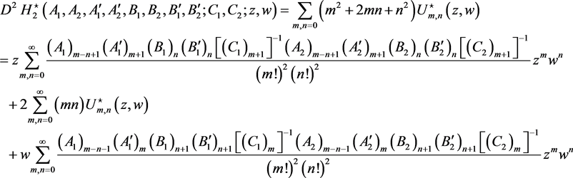
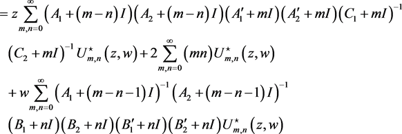
Operating with D on the Horn matrix function of two complex variables yields

$\begin{array}{c}D{H}_2={\displaystyle \underset{m,n=1}{\overset{\infty }{\sum }}}\frac{\left(m+n\right){\left(A\right)}_{m-n}{\left(A^{\prime }\right)}_m{\left(B\right)}_n{\left(B^{\prime }\right)}_n{\left[{\left(C\right)}_m\right]}^{-1}{\left[{\left(C^{\prime }\right)}_m\right]}^{-1}}{m!n!}{z}^m{w}^n\\ =zA{A}^{\prime }{C}^{-1}{H}_2\left(A+,A^{\prime }+,B,B^{\prime };C+;z,w\right)\\ +w{\left(A-I\right)}^{-1}B{B}^{\prime }{H}_2\left(A-,A^{\prime },B+,B^{\prime }+;C;z,w\right).\end{array}$ (30)

Operate with $d_1$ on the Horn matrix function, we obtain

$\begin{array}{c}{d}_1{H}_2={\displaystyle \underset{m=1,n=0}{\overset{\infty }{\sum }}}\frac{m{\left(A\right)}_{m-n}{\left(A^{\prime }\right)}_m{\left(B\right)}_n{\left(B^{\prime }\right)}_n{\left[{\left(C\right)}_m\right]}^{-1}}{m!n!}{z}^m{w}^n\\ =zA{A}^{\prime }{\left[C\right]}^{-1}{H}_2\left(A+I,A^{\prime }+I,B,B^{\prime };C+I;z,w\right),\end{array}$ (31)

$\begin{array}{c}{d}_1^{\left(2\right)}{H}_2={\displaystyle \underset{m=2,n=0}{\overset{\infty }{\sum }}}\frac{m\left(m-1\right){\left(A\right)}_{m-n}{\left(A^{\prime }\right)}_m{\left(B\right)}_n{\left(B^{\prime }\right)}_n{\left[{\left(C\right)}_m\right]}^{-1}{\left[{\left(C^{\prime }\right)}_n\right]}^{-1}}{m!n!}{z}^m{w}^n\\ =z^2{\left(A\right)}_2{\left(A^{\prime }\right)}_2{\left[{\left(C\right)}_2\right]}^{-1}{H}_2\left(A+2I,A^{\prime }+2I,B,B^{\prime };C+2I;z,w\right)\end{array}$ (32)

and

$\begin{array}{c}{d}_1^2{H}_2=d_1\left[A{A}^{\prime }{\left[C\right]}^{-1}{\displaystyle \underset{m,n=0}{\overset{\infty }{\sum }}}\frac{{\left(A+I\right)}_{m-n}{\left(A^{\prime }+I\right)}_m{\left(B\right)}_n{\left(B^{\prime }\right)}_n{\left[{\left(C+I\right)}_m\right]}^{-1}}{m!n!}{z}^{m+1}{w}^n\right]\\ =d_1^{\left(2\right)}{H}_2+d_1{H}_2\end{array}$

i.e.,

$d_1^{\left(2\right)}{H}_2-d_1\left(d_1-1\right)H_2=0.$ (33)

Similarly, for $d_2$ , we have

$d_2{H}_2=w{\left(A-I\right)}^{-1}B{B}^{\prime }{H}_2\left(A-I\mathrm{,}{A}^{\prime }\mathrm{,}B+I\mathrm{,}{B}^{\prime }+I\mathrm{<mo>\; ;\; </mo>}C\mathrm{<mo>\; ;\; </mo>}z\mathrm{,}w\right)\mathrm{,}$ (34)

$d_2^{\left(2\right)}{H}_2=w^2{\left[{\left(A-2I\right)}_2\right]}^{-1}{\left(B\right)}_2{\left(B^{\prime }\right)}_2{H}_2\left(A-2I,A^{\prime },B+2I,B^{\prime }+2I;C;z,w\right)$ (35)

and

$\begin{array}{c}{d}_2^2{H}_2=d_2\left[w{\left(A-I\right)}^{-1}B{B}^{\prime }{H}_2\left(A-I\mathrm{,}{A}^{\prime }\mathrm{,}B+I\mathrm{,}{B}^{\prime }+I\mathrm{<mo>\; ;\; </mo>}C\mathrm{<mo>\; ;\; </mo>}z\mathrm{,}w\right)\right]\\ =d_2^{\left(2\right)}{H}_2+d_2{H}_2\end{array}$ (36)

i.e.,

$\begin{array}{l}{d}_2^{\left(2\right)}{H}_2-d_2\left(d_2-1\right)H_2=0.\hfill \end{array}$ (37)

Hence the Horn matrix function $H_2\left(A\mathrm{,}{A}^{\prime }\mathrm{,}B\mathrm{,}{B}^{\prime }\mathrm{<mo>\; ;\; </mo>}C\mathrm{<mo>\; ;\; </mo>}z\mathrm{,}w\right)$ is a solution of the partial differential equations in the forms (33) and (37).

Now, we see that

$d_1{d}_2{H}_2=zwA{\left[\left(A-I\right)\right]}^{-1}{A}^{\prime }B{B}^{\prime }{\left[\left(C\right)\right]}^{-1}{H}_2\left(A,A^{\prime }+I,B+I,B^{\prime }+I;C+I;z,w\right).$ (38)

From (32), (35) and (38), we have

$\begin{array}{c}{D}^{\left(2\right)}{H}_2={\displaystyle \underset{m+n<2}{\overset{\infty }{\sum }}}\frac{{\left(A\right)}_{m-n}{\left(A^{\prime }\right)}_m{\left(B\right)}_n{\left(B^{\prime }\right)}_n{\left[{\left(C\right)}_m\right]}^{-1}}{m!n!}{z}^m{w}^n\\ +\left(d_1^{\left(2\right)}+2d_1{d}_2+d_2^{\left(2\right)}\right){\displaystyle \underset{m+n\ge 2}{\overset{\infty }{\sum }}}\frac{m{\left(A\right)}_{m-n}{\left(A^{\prime }\right)}_m{\left(B\right)}_n{\left(B^{\prime }\right)}_n{\left[{\left(C\right)}_m\right]}^{-1}}{m!n!}{z}^{m-1}{w}^n\end{array}$

$\begin{array}{l}=I+A{A}^{\prime }{\left[\left(C\right)\right]}^{-1}z+B{B}^{\prime }{\left[\left(A-I\right)\right]}^{-1}w\\ +{\left(A\right)}_2{\left(A^{\prime }\right)}_2{\left[{\left(C\right)}_2\right]}^{-1}{z}^2{H}_2\left(A+2I,A^{\prime }+2I,B,B^{\prime };C+2I;z,w\right)\\ +zwA{\left[\left(A-I\right)\right]}^{-1}{A}^{\prime }B{B}^{\prime }{\left[C\right]}^{-1}{H}_2\left(A,A^{\prime }+I,B+I,B^{\prime }+I;C+I;z,w\right)\\ +{\left[{\left(A-2I\right)}_2\right]}^{-1}{\left(B\right)}_2{\left(B^{\prime }\right)}_2{w}^2{H}_2\left(A-2I,A^{\prime },B+2I,B^{\prime }+2I;C;z,w\right).\end{array}$ (39)

The $\beta \left(D\right)$ -operator has been defined of two complex variables by Sayyed [28] in the form

$\beta \left(D\right)=1+{\displaystyle \underset{k=1}{\overset{N}{\sum }}}{D}^{\left(k\right)}$ (40)

where

$D^{\left(N\right)}=\{\begin{array}{l}{z}^N\frac{{\partial }^N}{\partial z^N}+\left(\begin{array}{c}N\\ 1\end{array}\right)z^{N-1}w\frac{{\partial }^N}{\partial z^{N-1}\partial w}+\left(\begin{array}{c}N\\ 2\end{array}\right)z^{N-2}{w}^2\frac{{\partial }^N}{\partial z^{N-2}\partial w^2}\\ +\cdots +w^N\frac{{\partial }^N}{\partial w^N};m+n\ge N\\ 1;\text{otherwise}.\end{array}$

where N is a finite positive integer.

We have by mathematical induction the following general form of differential operator $\beta \left(D\right)$ to Horn matrix function in the form

$\begin{array}{l}\beta \left(D\right)H_2=\left(1+{\displaystyle \underset{k=1}{\overset{N}{\sum }}}{D}^{\left(k\right)}\right)H_2\\ =H_2+{\displaystyle \underset{k=1}{\overset{N}{\sum }}}[{\displaystyle \underset{j=0}{\overset{k-1}{\sum }}}{\left(A\right)}_{k-j-1}{\displaystyle \underset{i=0}{\overset{j}{\sum }}}\frac{{\left[{\left(A-iI\right)}_i\right]}^{-1}{\left(A^{\prime }\right)}_{j-i}{\left(B\right)}_i{\left(B^{\prime }\right)}_i{\left[{\left(C\right)}_{j-i}\right]}^{-1}}{\left(j-i\right)!i!}{z}^{j-i}{w}^i\\ +{\displaystyle \underset{j=0}{\overset{k}{\sum }}}\left(\begin{array}{c}k\\ k-j\end{array}\right){\left(A\right)}_{k-j}{\left[{\left(A-jI\right)}_j\right]}^{-1}{\left(A^{\prime }\right)}_{k-j}{\left(B\right)}_j{\left(B^{\prime }\right)}_j{\left[{\left(C\right)}_{k-j}\right]}^{-1}{z}^{k-j}{w}^j\\ \begin{array}{c}\\ \\ \end{array}{H}_2\left(A+\left(k-2j\right)I,A^{\prime }+\left(k-j\right)I,B+jI,B^{\prime }+jI;C+\left(k-j\right)I;z,w\right)].\end{array}$ (41)

5. Hadamard Product of Two Horn’s Matrix Functions

Let $A_i,{A^{\prime }}_i,B_i,{B^{\prime }}_i$ and $C_i$ are commutative matrices in $C^{N\times N}$ such that $C_i+mI$ are invertible matrices for all integers $m\ge 0$ , $i=1,2$ .

The Hadamard product of two Horn’s matrix functions of two complex variables is defined in the form

$\begin{array}{l}{H}_2^{\star }\left(A_1,A_2,{A^{\prime }}_1,{A^{\prime }}_2{B}_1,B_2,{B^{\prime }}_1,{B^{\prime }}_2;C_1,C_2;z,w\right)\\ =H_2\left(A_1,{A^{\prime }}_1,B_1,{B^{\prime }}_1;C_1;z,w\right)\ast H_2\left(A_2,{A^{\prime }}_2,B_2,{B^{\prime }}_2;C_2;z,w\right)\\ ={\displaystyle \underset{m,n=0}{\overset{\infty }{\sum }}}\frac{{\left(A_1\right)}_{m-n}{\left({A^{\prime }}_1\right)}_m{\left(B_1\right)}_n{\left({B^{\prime }}_1\right)}_n{\left[{\left(C_1\right)}_m\right]}^{-1}{\left(A_2\right)}_{m-n}{\left({A^{\prime }}_2\right)}_m{\left(B_2\right)}_n{\left({B^{\prime }}_2\right)}_n{\left[{\left(C_2\right)}_m\right]}^{-1}}{{\left(m!\right)}^2{\left(n!\right)}^2}{z}^m{w}^n\\ ={\displaystyle \underset{m,n=0}{\overset{\infty }{\sum }}}{U}_{m,n}^{\star }\left(z,w\right)\end{array}$ (42)

where

$\begin{array}{l}{U}_{m,n}^{\star }\left(z,w\right)\\ =\frac{{\left(A_1\right)}_{m-n}{\left({A^{\prime }}_1\right)}_m{\left(B_1\right)}_n{\left({B^{\prime }}_1\right)}_n{\left[{\left(C_1\right)}_m\right]}^{-1}{\left(A_2\right)}_{m-n}{\left({A^{\prime }}_2\right)}_m{\left(B_2\right)}_n{\left({B^{\prime }}_2\right)}_n{\left[{\left(C_2\right)}_m\right]}^{-1}}{{\left(m!\right)}^2{\left(n!\right)}^2}{z}^m{w}^n\end{array}$

Now, we prove that the Hadamard product of two Horn’s matrix functions of two complex variables convergence for all z and w with $\left|z\right|<1$ and $\left|w\right|<1$ . If n is large enough, one can write $n\ge \Vert C_i\Vert$ , then the following relation is satisfied [7]

$\Vert {\left(C_i+nI\right)}^{-1}\Vert =\Vert \frac{1}{n}{\left(\frac{C_i}{n}+I\right)}^{-1}\Vert =\frac{1}{n}\Vert {\left(\frac{C_i}{n}+I\right)}^{-1}\Vert \le \frac{1}{n-\Vert C_i\Vert };n>\Vert C_i\Vert .$ (43)

Denote

${\gamma }_i\left(n\right)=\Vert {\left(C_i\right)}^{-1}\Vert \Vert {\left(C_i+I\right)}^{-1}\Vert \cdots \Vert {\left(C_i+\left(n-1\right)I\right)}^{-1}\Vert ;n>0.$ (44)

Note that

$\begin{array}{l}\Vert {\left(A_i\right)}_{m-n}\Vert \le {\left(\Vert A_i\Vert \right)}_{m-n}\mathrm{,}\Vert {\left({A^{\prime }}_i\right)}_m\Vert \le {\left(\Vert {A^{\prime }}_i\Vert \right)}_m\mathrm{,}\\ \Vert {\left(B_i\right)}_n\Vert \le {\left(\Vert B_i\Vert \right)}_n\mathrm{,}\Vert {\left({B^{\prime }}_i\right)}_n\Vert \le {\left(\Vert {B^{\prime }}_i\Vert \right)}_n\mathrm{.}\end{array}$ (45)

Then by relation (43)-(45) for m large enough, such that $m>\Vert C_i\Vert$ , it follows that

$\begin{array}{l}\underset{m\mathrm{,}n\to \infty }{lim}\left|\frac{\Vert U_{m+\mathrm{1,}n+1}^{\star }\left(z\mathrm{,}w\right)\Vert }{\Vert U_{m\mathrm{,}n}^{\star }\left(z\mathrm{,}w\right)\Vert }\right|\\ \le \underset{m\mathrm{,}n\to \infty }{lim}\left|\frac{\left(\Vert {A^{\prime }}_1\Vert +m\right)\left(\Vert B_1\Vert +n\right)\left(\Vert {B^{\prime }}_1\Vert +n\right)\left(\Vert {A^{\prime }}_2\Vert +m\right)\left(\Vert B_2\Vert +n\right)\left(\Vert {B^{\prime }}_2\Vert +n\right)}{{\left(m+1\right)}^2{\left(n+1\right)}^2\left(m-\Vert C_1\Vert \right)\left(m-\Vert C_2\Vert \right)}\right|\left|z\right|\left|w\right|\\ =0\text{for}\text{all}\left|z\right|<1\text{and}\left|w\right|<1.\end{array}$ (46)

Thus, the power matrix series (42) is convergent for all complex numbers $\left|z\right|<1$ and $\left|w\right|<1$ .

From relation (17) and the conditions (19) and (20), we can write

$\begin{array}{l}{H}_2^{\star }\left(A_1,A_2,{A^{\prime }}_1,{A^{\prime }}_2,B_1,B_2,{B^{\prime }}_1,{B^{\prime }}_2;C_1,C_2;z,w\right)\\ ={\displaystyle \underset{m,n=0}{\overset{\infty }{\sum }}}\frac{{\left(A_1\right)}_{m-n}{\left(A_2\right)}_{m-n}{\left(B_1\right)}_n{\left(B_2\right)}_n{\left({B^{\prime }}_1\right)}_n{\left({B^{\prime }}_2\right)}_n{\Gamma }^{-1}\left({A^{\prime }}_1\right){\Gamma }^{-1}\left(C_1-{A^{\prime }}_1\right){\Gamma }^{-1}\left({A^{\prime }}_2\right){\Gamma }^{-1}\left(C_2-{A^{\prime }}_2\right)}{{\left(m!\right)}^2{\left(n!\right)}^2}\\ \left({\displaystyle {\int }_0^1}{\displaystyle {\int }_0^1}{t}^{{A^{\prime }}_1+\left(m-1\right)I}{s}^{{A^{\prime }}_2+\left(m-1\right)I}{\left(1-t\right)}^{C_1-{A^{\prime }}_1-I}{\left(1-s\right)}^{C_2-{A^{\prime }}_2-I}\text{d}t\text{d}s\right)\Gamma \left(C_1\right)\Gamma \left(C_2\right)z^m{w}^n\\ ={\Gamma }^{-1}\left({A^{\prime }}_1\right){\Gamma }^{-1}\left({A^{\prime }}_2\right){\Gamma }^{-1}\left(C_1-{A^{\prime }}_1\right){\Gamma }^{-1}\left(C_2-{A^{\prime }}_2\right)\Gamma \left(C_1\right)\Gamma \left(C_2\right)\\ {\displaystyle {\int }_0^1}{\displaystyle {\int }_0^1}H\left(A_1,A_2,B_1,B_2,{B^{\prime }}_1,{B^{\prime }}_2;-,-;tsz,w\right)t^{{A^{\prime }}_1-I}{s}^{{A^{\prime }}_2-I}{\left(1-t\right)}^{C_1-{A^{\prime }}_1-I}{\left(1-s\right)}^{C_2-{A^{\prime }}_2-I}\text{d}t\text{d}s\end{array}$ (47)

where

$\begin{array}{l}H\left(A_1,A_2,B_1,B_2,{B^{\prime }}_1,{B^{\prime }}_2;-,-;z,w\right)\\ ={\displaystyle \underset{m,n=0}{\overset{\infty }{\sum }}}\frac{{\left(A_1\right)}_{m-n}{\left(A_2\right)}_{m-n}{\left(B_1\right)}_n{\left(B_2\right)}_n{\left({B^{\prime }}_1\right)}_n{\left({B^{\prime }}_2\right)}_n}{{\left(m!\right)}^2{\left(n!\right)}^2}{z}^m{w}^n.\end{array}$

Therefore, an integral representation for Hadamard product of two Horn’s matrix functions is obtained.

Contiguous Functions Relation for Hadamard Product of Two Horn’s Matrix Functions

For the Hadamard product of two Horn’s matrix functions $H_2^{\star }\left(A_1\mathrm{,}{A}_2\mathrm{,}{B}_1\mathrm{,}{B}_2\mathrm{,}{B^{\prime }}_1\mathrm{,}{B^{\prime }}_2\mathrm{<mo>\; ;\; </mo>}{C}_1\mathrm{,}{C}_2\mathrm{<mo>\; ;\; </mo>}z\mathrm{,}w\right)$ , we can define the contiguous function relations as follows

$\begin{array}{l}{H}_2^{\star }\left(A_i+\right)\mathrm{<mo>\; =\; </mo>}{A}_i^{-1}{\displaystyle \underset{m\mathrm{,}n\mathrm{<mo>\; =\; </mo>0}}{\overset{\infty }{\sum }}}\left(A_i+\left(m-n\right)I\right)U_{m\mathrm{,}n}^{\star }\left(z\mathrm{,}w\right)\mathrm{,}\hfill \end{array}$ (48)

$H_2^{\star }\left(A_i-\right)={\displaystyle \underset{m,n=0}{\overset{\infty }{\sum }}}\left(A_i-I\right){\left(A_i+\left(m-n-1\right)I\right)}^{-1}{U}_{m,n}^{\star }\left(z,w\right),$ (49)

$H_2^{\star }\left({A^{\prime }}_i+\right)={A^{\prime }}_i{}^{-1}{\displaystyle \underset{m,n=0}{\overset{\infty }{\sum }}}\left({A^{\prime }}_i+mI\right)U_{m,n}^{\star }\left(z,w\right),$ (50)

$H_2^{\star }\left({A^{\prime }}_i-\right)={\displaystyle \underset{m,n=0}{\overset{\infty }{\sum }}}\left({A^{\prime }}_i-I\right){\left({A^{\prime }}_i+\left(m-1\right)I\right)}^{-1}{U}_{m,n}^{\star }\left(z,w\right),$ (51)

$H_2^{\star }\left(B_i+\right)={\displaystyle \underset{m,n=0}{\overset{\infty }{\sum }}}{B}_i^{-1}\left(B_i+nI\right)U_{m,n}^{\star }\left(z,w\right),$ (52)

$H_2^{\star }\left(B_i-\right)={\displaystyle \underset{m,n=0}{\overset{\infty }{\sum }}}\left(B_i-I\right){\left(B_i+nI\right)}^{-1}{U}_{m,n}^{\star }\left(z,w\right),$ (53)

$H_2^{\star }\left({B^{\prime }}_i+\right)={\displaystyle \underset{m,n=0}{\overset{\infty }{\sum }}}{B^{\prime }}_i{}^{-1}\left({B^{\prime }}_i+nI\right)U_{m,n}^{\star }\left(z,w\right),$ (54)

$H_2^{\star }\left({B^{\prime }}_i-\right)={\displaystyle \underset{m,n=0}{\overset{\infty }{\sum }}}\left({B^{\prime }}_i-I\right){\left({B^{\prime }}_i+nI\right)}^{-1}{U}_{m,n}^{\star }\left(z,w\right),$ (55)

$H_2^{\star }\left(C_i+\right)={\displaystyle \underset{m,n=0}{\overset{\infty }{\sum }}}\left(C_i+I\right){\left(C_i+mI\right)}^{-1}{U}_{m,n}^{\star }\left(z,w\right)$ (56)

and

$H_2^{\star }\left(C_i-\right)={\displaystyle \underset{m,n=0}{\overset{\infty }{\sum }}}{\left(C_i-I\right)}^{-1}\left(C_i+mI\right)U_{m,n}^{\star }\left(z,w\right).$ (57)

For all integers $k\ge 1$ and $i=1,2$ we deduce that

$\begin{array}{l}{H}^{\star }\left(A_i+kI\right)\\ ={\displaystyle \underset{r=1}{\overset{k}{\prod }}}{\left(A_i+\left(r-1\right)I\right)}^{-1}{\displaystyle \underset{m,n=0}{\overset{\infty }{\sum }}}{\displaystyle \underset{r=1}{\overset{k}{\prod }}}\left(A_i+\left(m-n+\left(r-1\right)\right)I\right)U_{m,n}^{\star }\left(z,w\right),\end{array}$ (58)

$H^{\star }\left(A_i-kI\right)={\displaystyle \underset{r=1}{\overset{k}{\prod }}}\left(A_i-rI\right){\displaystyle \underset{m,n=0}{\overset{\infty }{\sum }}}{\displaystyle \underset{r=1}{\overset{k}{\prod }}}{\left(A_i+\left(m-n-r\right)I\right)}^{-1}{U}_{m,n}^{\star }\left(z,w\right),$ (59)

$H^{\star }\left({A^{\prime }}_i+kI\right)={\displaystyle \underset{r=1}{\overset{k}{\prod }}}{\left({A^{\prime }}_i+\left(r-1\right)I\right)}^{-1}{\displaystyle \underset{m,n=0}{\overset{\infty }{\sum }}}{\displaystyle \underset{r=1}{\overset{k}{\prod }}}\left({A^{\prime }}_i+\left(m+\left(r-1\right)\right)I\right)U_{m,n}^{\star }\left(z,w\right),$ (60)

(61)

(62)

(63)

(64)

(65)

(66)

and

(67)

The Hadamard product of two Horn’s matrix functions is affected by the differential operator D, so, for all, we obtain that

(68)

(69)

(70)

(71)

and

(72)

Next, let us operate with D on (5.1) on both sides, we obtain

(73)

Hence, we can find that

6. Conclusion

The results are established in this study to express a clear idea that the use of operational techniques provides a simple and straightforward method to get new relations for Horn matrix functions. Therefore, these results are considered original, variant, significant, interesting and capable to develop its study in the future.

Acknowledgements

1) The authors would like to thank the referees for their valuable comments and suggestions to improve the quality of the paper.

2) The third Author (Ayman Shehata) expresses his sincere appreciation to Dr. Mohammed Eltayeb Elffaki Elasmaa (Assistant Prof. Department of English language, Faculty of Arts and Human Studies, University of Dongola, Sudan) for his kinds interests, encouragements, help and correcting language errors for this paper.

Open Problem

The same class of new differential and integral operators can be used for the Horn matrix functions. Hence, new results and further applications can be obtained. Further applications will be discussed in a forthcoming paper.

Conflicts of Interest

The authors declare no conflicts of interest.

References

[1]	Constantine, A.G. and Mairhead, R.J. (1972) Partial Differential Equations for Hypergeometric Functions of Two Argument Matrices. Journal of Multivariate Analysis, 2, 332-338. https://doi.org/10.1016/0047-259X(72)90020-6
[2]	James, A.T. (1975) Special Functions of Matrix and Single Argument in Statistics in Theory and Application of Special Functions. In: Askey, R.A., Ed., Academic Press, New York.
[3]	Erdélyi, A., Magnus, W., Oberhettinger, F. and Tricomi, F.G. (1953) Higher Tanscendental Functions. McGraw-Hill Book Co., New York.
[4]	Mathai, A.M. (1993) A Handbook of Generalized Special Functions for Statistical and Physical Sciences. Oxford University Press, Oxford.
[5]	Mathai, A.M. (1997) Jacobians of Matrix Transformations and Functions of Matrix Argument. World Scientific Publishing, New York. https://doi.org/10.1142/3438
[6]	Jódar, L. and Cortés, J.C. (1998) On the Hypergeometric Matrix Function. Journal of Computational and Applied Mathematics, 99, 205-217. https://doi.org/10.1016/S0377-0427(98)00158-7
[7]	Jódar, L. and Cortés, J.C. (2000) Closed Form General Solution of the Hypergeometric Matrix Differential Equation. Mathematical and Computer Modelling, 32, 1017-1028. https://doi.org/10.1016/S0895-7177(00)00187-4
[8]	Sayyed, K.A.M., Metwally, M.S. and Mohamed, M.T. (2009) Certain Hypergeometric Matrix Function. Scientiae Mathematicae Japonicae, 69, 315-321. http://www.jams.or.jp/notice/scmjol/2009.html2009-21
[9]	Khammash, G.S. and Shehata, A. (2012) A Study on Some Prop-erties of Legendre Polynomials and Integral Transforms. International Journal of Open Problems in Computer Science and Mathe-matics (IJOPCM), 5, 1-6. https://doi.org/10.12816/0006100
[10]	Khammash, G.S. and Shehata, A. (2012) On Humbert Matrix Polynomials. Asian Journal of Current Engineering and Maths (AJCEM), 1, 232-240.
[11]	Metwally, M.S. (2011) On p-Kummers Matrix Function of Complex Variable under Differential Operators and Their Properties. Southeast Asian Bulletin of Mathematics, 35, 1-16.
[12]	Metwally, M.S., Mohamed, M.T. and Shehata, A. (2008) On Hermite-Hermite Matrix Polynomials. Mathematica Bohemica, 133, 421-434.
[13]	Metwally, M.S. and Shehata, A. (2013) A Study of a New Properties of Hermite-Hermite Matrix Polynomials and Their Applications. International Journal of Mathematical Sciences and Engineering Applications (IJMSEA), 7, 19-33.
[14]	Rashwan, R.A., Metwally, M.S., Mohamed, M.T. and Shehata, A. (2013) Certain Kummer’s Matrix Function of Two Complex Variables under Certain Differential and Integral Operators. Thai Journal of Mathematics, 11, 725-740.
[15]	Shehata, A. (2012) A New Extension of Hermite-Hermite Matrix Polynomials and Their Properties. Thai Journal of Mathematics, 10, 433-444.
[16]	Shehata, A. (2012) A New Extension of Gegenbauer Matrix Polynomials and Their Properties. Bulletin of International Mathematical Virtual Institute, 2, 29-42.
[17]	Shehata, A. (2012) On Pseudo Legendre Matrix Polynomials. International Journal of Mathematical Sciences and Engineering Applications, 6, 251-258.
[18]	Upadhyaya, L.M. and Shehata, A. (2011) On Legendre Matrix Polynomials and Its Applications. International Transactions in Mathematical Sciences and Computer, 4, 291-310.
[19]	Shehata, A. (2011) On p and q-Horn’s Matrix Function of Two Complex Variables. Applied Mathematics, 2, 1437-1442. https://doi.org/10.4236/am.2011.212203
[20]	Shehata, A. (2013) Certain pl(m,n)-Kummer Matrix Function of Two Complex Variables under Differential Operator. Applied Mathematics, 4, 91-96. https://doi.org/10.4236/am.2013.41016
[21]	Horn, J. (1931) Hypergeometrische Funktionen zweier Veränderlichen. Mathematische Annalen, 105, 381-407. https://doi.org/10.1007/BF01455825
[22]	Horn, J. (1935) Hypergeometrische Funktionen zweier Veränderlichen. Mathematische Annalen, 111, 638-677. https://doi.org/10.1007/BF01472246
[23]	Horn, J. (1936) Hypergeometrische Funktionen zweier Veränderlichen. Mathematische Annalen, 113, 242-291. https://doi.org/10.1007/BF01571633
[24]	Horn, J. (1938) Hypergeometrische Funktionen zweier Veränderlichen im Schnittpunkt dreier Singularitäten. Mathematische Annalen, 115, 435-455. https://doi.org/10.1007/BF01448950
[25]	Jódar, L. and Cortés, J.C. (1998) Some Properties of Gamma and Beta Matrix Functions. Applied Mathematics Letters, 11, 89-93. https://doi.org/10.1016/S0893-9659(97)00139-0
[26]	Dunford, N. and Schwartz, J.T. (1957) Linear Operators, Part I, General Theory. Interscience Publishers, Inc., New York.
[27]	Shehata, A. (2009) A Study of Some Special Functions and Polynomials of Complex Variables. PhD Thesis, Assiut University, Assiut.
[28]	Sayyed, K.A.M. (1975) Basic Sets of Polynomials of Two Complex Variables and Convergence Propertiess. PhD Thesis, Assiut University, Assiut.