1. Introduction
Although spectral analysis is one of the oldest tools for time series analysis, it is still one of the most widely used analysis techniques in many branches of sciences, [1] - [6] . For zero mean r-vector valued strictly stationary time series, the spectral estimation has been studied, [7] - [17] . Time series with missing observations frequantly appear in paractice. If a block of observations is periodically unobtainable, Jones [18] provides a development for spectral estimation of a stationary time series. The theory of amplitude-modulated stationary processes has been developed by Parzen [19] and applied to periodic missing observations problems [20] . The case where an observation is made or not according to the out come of a Bernoulli trial has been discussed by Scheinok [21] . Bloomfield [22] considered the case where a more general random mechanism is involved. Broersen et al. [23] and [24] developed models for time series with missing observation and discussed their use for spectral estimation. Unbiased spectral estimators have been formulated assuming wavelet models of stationary time series by [25] . Their asymptotic properties have been also investigated.
In this paper, we will discuss the spectral analysis of a strictly stationary r-vector valued continuous time series with randomly missing observations in joint segments of observations. The paper is organized as follows. Section 2 introduces the basic definitions and assumptions. The modified series is defined in Section 3. Section 4 considers the expanded finite Fourier transform and its properties. The modified periodogram, the spectral density estimator and its properties are given in Section 5.
2. Observed Series
Let  be a zero mean r-vector valued strictly stationary time series with
 (2.1)
(2.1)
and
 (2.2)
(2.2)
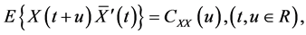
where  denotes the matrix of absolute values, the bar denotes the complex conjugate and '
 ' denotes the matrix transpose. We may then define
  the
the  matrix of second order spectral densities by
 (2.3)
(2.3)
Using the assumed stationary, we then set down
Assumption I.  is a strictly stationary continuous series all of whose moments exist. For each
  and any k-tuple
  we have
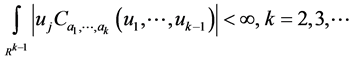 (2.4)
(2.4)
where
 (2.5)
(2.5)
( ;
; ).
).
Because cumulants are measures of the joint dependence of random variables, (2.4) is seen to be a form of mixing or asymptotic independence requirement for values of  well separated in time. If
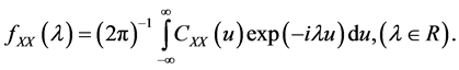
  satisfies Assumption I we may define its cumulant spectral densities by
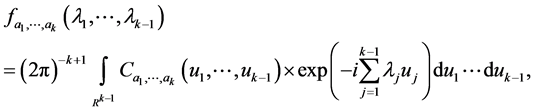 (2.6)
(2.6)
(![]() ). If
). If ![]() the cross-spectra
the cross-spectra ![]() are collected together in the matrix
are collected together in the matrix ![]() of (2.3).
of (2.3).
Assumption II. Let ![]() is bounded, is of bounded variation
is bounded, is of bounded variation
and vanishes for all t outside the interval![]() , that is called data window.
, that is called data window.
3. Modified Series
Let ![]() be a process independent of
be a process independent of ![]() such that, for every t
such that, for every t
![]()
note that
![]()
The success of recording an observation not depend on the fail of another and so it is independent. We may then define the modified series
![]()
with components,
![]()
where
![]()
4. Expanded Finite Fourier Transform in L-Joint Segments of Observations
In the case when there are some randomly missing observations, Elhassanein [17] constructed the expanded finite Fourier transform on disjoint segments of observations. In this section the expanded finite Fourier transform is constructed in L-joint segments of observations for a strictly stationary r-vector valued time series. Expression for its mean, variance and cumulant will be derived. The results introduced here may be regarded as a generalization to [13] and [17] . Let ![]() be an observed stretch of data with some randomly missing observations. Let
be an observed stretch of data with some randomly missing observations. Let![]() , where L is the number of joint segments and N is the length of each segment and M is the length of joint parts,
, where L is the number of joint segments and N is the length of each segment and M is the length of joint parts, ![]() , where
, where ![]() we get the results in [17] . The expanded finite Fourier transform of a given stretch of data, is defined by
we get the results in [17] . The expanded finite Fourier transform of a given stretch of data, is defined by
![]() (4.1)
(4.1)
where ![]() and
and ![]() is the data window satisfies Assump- tion II.
is the data window satisfies Assump- tion II.
Theorem 4.1. Let ![]() be a strictly stationary r-vector valued time series with mean zero, and satisfy Assumption I. Let
be a strictly stationary r-vector valued time series with mean zero, and satisfy Assumption I. Let ![]() be defined as (3.1), and
be defined as (3.1), and ![]() satisfy Assumption II, for
satisfy Assumption II, for ![]() then
then
![]() (4.2)
(4.2)
![]() (4.3)
(4.3)
where
![]()
and
![]()
where
![]()
for ![]() then
then
![]() (4.4)
(4.4)
![]()
(4.5)
where ![]() is uniform in
is uniform in ![]() as
as![]() ,
, ![]() and
and
![]()
Proof. We will prove (4.5), by (4.1) we get
![]()
let ![]() and since
and since
![]()
for some constants ![]() and
and![]() , we get
, we get
![]()
where
![]()
since ![]() satisfy Assumption II for
satisfy Assumption II for ![]() then
then
![]()
which implies to![]() , using (2.6) the proof is completed. ,
, using (2.6) the proof is completed. ,
5. Estimation
Using expanded finite Fourier transform (4.1), we construct the modified periodogram as
![]() (5.1)
(5.1)
such that
![]()
where the bar denotes the complex conjugate. The smoothed spectral density estimate is constructed as
![]() (5.2)
(5.2)
Theorem 5.1. Let ![]() be a strictly stationary r-vector valued continuous time series with mean zero, and satisfy Assumption I. Let
be a strictly stationary r-vector valued continuous time series with mean zero, and satisfy Assumption I. Let ![]() be given by (3.6), and
be given by (3.6), and ![]() satisfy Assumption II for
satisfy Assumption II for ![]() then
then
![]() (5.3)
(5.3)
![]() (5.4)
(5.4)
![]() (5.5)
(5.5)
where the summation extends over all partitions
![]() into pairs of the quantities
into pairs of the quantities
![]() excluding the case with
excluding the case with ![]() for some
for some![]() , where
, where ![]() is uniform in
is uniform in![]() .
.
Proof. By (5.1), we have
![]()
then by (4.3) the proof of (5.3) is completed. From (5.1), and by Theorem (2.3.2) in [10] p. 21, we have
![]()
By Theorem (4.1) the proof of (5.4) is completed. From (5.1), we have
![]()
By Theorem (2.3.2) in [10] p. 21, we get
![]()
where the summation extends over all indecomposable partitions ![]()
![]()
![]() of the transformed table
of the transformed table
![]()
Then, by Theorem (4.1), we get the proof of (5.5). ,
Theorem 5.2. Let ![]() be a strictly stationary r-vector valued time series
be a strictly stationary r-vector valued time series
with mean zero, and satisfy Assumption I. Let ![]() be
be
given by (3.6), ![]() for
for ![]() and
and ![]() satisfy Assumption II for
satisfy Assumption II for ![]() Then
Then ![]() are asymptotically independent
are asymptotically independent ![]() variates. Also if
variates. Also if![]() . then
. then ![]() is asymptotically
is asymptotically ![]() independent of the previous variates. Where,
independent of the previous variates. Where, ![]() denotes an
denotes an ![]() symmetric matrix-valued Wishart variate with covariance matrix
symmetric matrix-valued Wishart variate with covariance matrix ![]() and
and ![]() degree of freedom and
degree of freedom and ![]() denotes an
denotes an ![]() Hermitian matrix-valued complex Wishart variate with covariance matrix
Hermitian matrix-valued complex Wishart variate with covariance matrix ![]() and
and ![]() degree of freedom.
degree of freedom.
Proof. The proof comes directly from Theorem (4.2), for more details about Wishart distribution see [26] . ,
Theorem 5.3. Let ![]() be a strictly stationary r-vector valued time series with mean zero, and satisfy Assumption I. Let
be a strictly stationary r-vector valued time series with mean zero, and satisfy Assumption I. Let ![]() be given by (3.7),
be given by (3.7), ![]() then
then
![]() (5.6)
(5.6)
![]() (5.7)
(5.7)
Proof. By (5.2), we have
![]()
then by (5.3) the proof of (5.6) is completed. From (5.2), we get
![]()
which completes the proof of (5.7). ,
Theorem 5.4. Let ![]() be a strictly stationary r-vector valued time series with mean zero, and satisfy Assumption I. Let
be a strictly stationary r-vector valued time series with mean zero, and satisfy Assumption I. Let ![]() be given by (5.2),
be given by (5.2),
![]() ,
, ![]() for
for![]() , Then
, Then
![]() are asymptotically independent
are asymptotically independent ![]() variates. Also if
variates. Also if![]() . then
. then ![]() is asymptotically
is asymptotically ![]() indepen- dent of the previous variates.
indepen- dent of the previous variates.
Proof. The proof comes directly by Theorem (5.3) and Theorem (7.3.2) in [26] p. 162. ,