Internal Vibration and Synchronization of Four Coupled Self-Excited Elastic Beams ()
Received 6 July 2016; accepted 20 August 2016; published 23 August 2016

1. Introduction
Vibration of elastic beams is an important issue given that failure by fatigue in mechanical systems may arise. The majority of the reports published on this topic are aimed to the analysis of vibration modes [1] - [4] or resonance [5] . Particularly, vibration of beams exposed to the Vortex Induced Vibration (VIV) phenomenon, e.g. parts in rotary machines and marine structures, is rarely studied. VIV is part of the fluid-structure problem, and it arises when shedding vortices apply oscillatory forces on cylinders or beams in the direction perpendicular to both the flow and the structure: the beams oscillate due to these forces [6] . In [7] , VIV in a single beam is modeled by adding a nonlinear self-oscillation term to the governing equation, and the self-oscillation parameter is varied in order to cover from linear to nonlinear behavior. Multiple frequencies of the nonlinear beam are reported using the power spectra of the time series of the free-end transverse displacements. Then, as in [7] , a beam subject to VIV can be considered as a spatially extended oscillator described by partial differential equations.
The collective behavior, particularly synchronization, of spatially extended coupled oscillators has been poorly studied in the past. Nowadays, the majority of the reports on the collective behavior of coupled oscillators are focused on oscillators described by ordinary differential equations, e.g. [8] [9] . However, the works on the coupled behavior of spatially extended systems described through partial differential equations are increasing [10] - [13] . The behavior of four coupled elastic beams subject to VIV has been analyzed in [14] [15] . In [14] the collective behavior of four coupled self-excited elastic beams is numerically studied. Self-excitation is modeled by adding a van der Pol damping term. Coupling based on shared boundary conditions at the roots of the beams is proposed, and the influence of the coupling parameter on the collective dynamics is analyzed. The synchronization among beams is studied using correlation coefficients, and the multiple frequencies of the beam tip vibration are determined through the power spectra of the transverse displacement time series. The oscillation death (OD) phenomenon in the coupled beams of [14] is studied in [15] . It is reported that OD arises when the coupling matrix becomes singular.
In this work, the vibration behavior along the length of a single beam and the synchronization among internal points of four coupled self-excited elastic beams are numerically studied. The transverse displacements of three internal points along the length plus the tip of each beam are monitored, and the power spectra of the resulting time series are employed to determine the oscillation frequencies. The synchronization between pairs of beams is studied by means of the corresponding phase portraits and correlation coefficients of the time series of each monitoring point. As in [14] , coupling through the root of the beams is considered. To obtain the time series of the transverse displacements, the set of coupled governing partial differential equations is numerically solved using the finite differences method.
2. Mathematical Model and Coupling
The complete derivation of the mathematical model can be found in [14] . Here, just the main equations are showed. The transversal motion of a clamped thin beam of fixed transversal section, homogeneous material, constant properties and no external loads (see Figure 1) is governed by the dimensionless equation
 (1)
(1)
where X is the distance from the root, Y(X, τ) is the transverse displacement, and τ is the time. As in [14] , a van der Pol term is added to Equation (1) in order to consider the VIV phenomenon and the fluid-structure interaction:
 (2)
(2)
![]()
Figure 1. Coordinate system in a single beam.
where A is a constant which rules the self-excited oscillations. Assuming that there are four beams, Equation (2) is rewritten as
 (3)
(3)
where i = 1, 2, 3, 4. As in [14] , coupling through the root of the beams is considered (see Figure 2). Each uncoupled beam is subject to the boundary conditions [16]
 (4)
(4)
 (5)
(5)
 . (6)
. (6)
The remaining boundary condition must consider the coupled nature of the beams. The displacements at the roots of beams are null, so the coupling through the slopes of the beams at the roots is considered [14] . Then,
 (7)
(7)
where K is the coupling parameter. Equation (7) can form a linear system as follows:
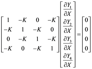 . (8)
. (8)
The matrix of Equation (8) represents a coupling matrix, and is named here as K. It is verified that . Whenever det(K) ≠ 0, the four boundary conditions given by Equation (7) are linearly independent. On the contrary, if det(K) = 0, K becomes singular for K = ±0.5 and in this case the oscillation death
![]()
Figure 2. Four beams coupled through the roots on the same shaft [14] . The dimensionless length of every beam is equal to 1.
phenomenon of beams may arise [15] .
3. Numerical Solution
For the sake of simplicity, the finite differences method was selected to numerically solve the mathematical model of the coupled beams. The explicit finite difference schemes reported in [17] were employed for the discretization of the partial differential equations and the corresponding boundary conditions. For numerical stability, in the computer simulations the following dimensionless values were used for the spatial grid and the time step, respectively: ΔX = 0.005, Δτ = 1.0 ´ 10−6. To prevent undesired transient solutions, computer runs were carried out for long dimensionless integration times, e.g. τ = 10,000. The initial conditions of the four beams were as follows: X1 = 1, Y1 = 0, X2 = 0, Y2 = 1, X3 = 1, Y3 = 1, X4 = 0, Y4 = 0.
Fortran programming language was employed to create the computer program. The computer runs aim to analyze the influence of A, the self-oscillation constant, on the coupled behavior of the beams. Three values of A are considered: 0.1, 0.5 and 1.0, which cover from linear to nonlinear behavior of the self-excited beams. To test the internal synchronization, four monitoring points in the X coordinate of each beam were selected: XA = 0.0965, XB = 0.50, XC = 0.8846 and XD = 1.0. To simulate a weak coupling, during the computer runs the value of the coupling parameter was kept constant at 0.1, i.e. K = 0.1.
4. Results and Comments
Given the large amount of data generated by the computer runs, and considering that the vibration behavior of the four beams are qualitatively similar, the time series and the power spectra presented here are just for the beam 1 of Figure 2 using the values of the self-oscillating constant defined in the preceding Section. The coupled behavior of the four beams is analyzed through the phase portraits and the correlation coefficients of the time series of the monitors obtained for all of the possible beam combinations.
Figures 3-5 show the time series of the transverse displacement for the monitors XA, XB, XC and XD of beam 1 for the considered values of the self-oscillating constant, i.e. A = 0.1, A = 0.5 and A = 1.0, respectively. Figure 3(a) and Figure 3(c) show that for A = 0.1 the time series of the XA and XC monitoring points exhibit a similar oscillation pattern: a dynamic behavior in which a dominant high frequency wave (3615.78 Hz) is enveloped by a low frequency one (19.59 Hz). The values of these frequencies were obtained through the power spectra depicted in Figure 6(a) and Figure 6(c), obtained from the corresponding time series. For A = 0.5, the time series of the XA and XC monitors are shown in Figure 4(a) and Figure 4(c). In this case the high frequency has a value of 3596.89 Hz, whereas the low one has a value of 13.35 Hz. These values are shown in the power spectra of Figure 7(a) and Figure 7(c). The XB and XD monitoring points of the beam 1 share an analogous oscillation pattern for A = 0.1 and A = 0.5: a low frequency dominant component (19.59 Hz for A = 0.1, and 13.35 Hz for A = 0.5), and a high frequency component which was undetectable by the power spectra: see Figure 6(b) and Figure 6(d) for A = 0.1 and Figure 7(b) and Figure 7(d) for A = 0.5.
The time series of the transverse displacements monitoring points for A = 1.0 are shown in Figure 5. The XA and XB monitors (see Figure 5(a) and Figure 5(b), respectively) exhibit an oscillation pattern in which a high frequency dominant component (3667.5 Hz) is enveloped by a low frequency one (67.06 Hz). However, some remarkable differences are detected between these two waves: the amplitude of the XA monitor wave has a value of 3, whereas the amplitude of the XB monitor wave has a value of 2. Besides, the power of the low frequency component of the XA monitor is larger than the power of the low frequency component of the XB monitor, as is observed in the power spectra of Figure 8(a) and Figure 8(b), respectively. In accordance to the time series of Figure 5(c) and the corresponding power spectrum of Figure 8(c), the XC monitoring point shows an inverse oscillation pattern related to the XA and XB monitors: a low frequency dominant pattern (67.0 Hz) and a high frequency (3667.5 Hz) weak component. For its part, the XD monitor exhibits a single low frequency component of 67.06 Hz, as is shown in the time series of Figure 5(d) and in the power spectrum of Figure 8(d).
The coupled vibration behavior of the beams is analyzed by means of phase portraits and correlation coefficients, which were obtained from the time series of the transverse displacements monitoring points. Figure 9 shows the phase portraits between pair of beams for A = 0.1, considering the time series of the transverse displacements in the XA monitor. Adjacent pairs of beams 1 - 2 (Figure 9(a)), 1 - 4 (Figure 9(c)), 2 - 3 (Figure 9(d)) and 3 - 4 (Figure 9(f)) exhibit phase portraits which correspond to time series with anti-phase synchronization but different amplitudes of the transverse displacement [18] . The correlation coefficients corresponding to
![]()
Figure 3. Time series of the transverse displacement monitoring points of beam 1 for A = 0.1. Monitoring points: (a) XA, (b) XB, (c) XC, (d) XD.
![]()
Figure 4. Time series of the transverse displacement monitoring points of beam 1 for A = 0.5. Monitoring points: (a) XA, (b) XB, (c) XC, (d) XD.
![]()
Figure 5. Time series of the transverse displacement monitoring points of beam 1 for A = 1.0. Monitoring points: (a) XA, (b) XB, (c) XC, (d) XD.
![]()
Figure 6. Power spectra corresponding to the time series of Figure 3.
![]()
Figure 7. Power spectra corresponding to the time series of Figure 4.
![]()
Figure 8. Power spectra corresponding to the time series of Figure 5.
![]()
Figure 9. Phase portraits between pairs of beams for the time series of the XA monitor for A = 0.1.
the above pair of beams have a value of −0.7670, as is shown in the first column of Table 1. The pairs of beams 1 - 3 (Figure 9(b)) and 2 - 4 (Figure 9(e)), which are not adjacent in the shaft, exhibit complete synchronization [18] . This dynamic condition is reflected in the value of 1 for their correlation coefficients, depicted in Table 1.
The phase portraits and the correlation coefficients for A = 0.5 and the XA monitor are shown in Figure 10 and Table 2, respectively. Adjacent pairs of beams such as 1 - 2 (Figure 10(a)), 1 - 4 (Figure 10(c)), 2 - 3 (Figure
![]()
Figure 10. Phase portraits between pairs of beams for the time series of the XA monitor for A = 0.5.
10(d)) and 3 - 4 (Figure 10(f)), present small anti-phase synchronization with different amplitudes of the transverse displacement, which is corroborated with a value of the correlation coefficient of −0.0667. Not-adjacent
![]()
Table 1. Dimensionless correlation coefficients between beams for A = 0.1.
![]()
Table 2. Dimensionless correlation coefficients between beams for A = 0.5.
pairs of beams, i.e. 1 - 3 (Figure 10(b)) and 2 - 4 (Figure 10(e)), present full synchronization, as is corroborated by their correlation coefficients with a value of 1.
The phase portraits between the diverse pair of beams for A = 1.0 and the XA monitor are displayed in Figure 11. The pairs of beams 1 - 2 (Figure 11(a)) and 3 - 4 (Figure 11(f)) present small anti-phase synchronization with correlation coefficients of −0.0730 shown in the first column of Table 3. The pairs of beams 1 - 4 (Figure 11(c)) and 2 - 3 (Figure 11(d)) exhibit small phase synchronization, and their correlation coefficients have a value of 0.0804. Besides, for A = 1.0, the not-adjacent pairs 1 - 3 (Figure 11(b)) and 2 - 4 (Figure 11(e)) undergo anti-phase synchronization with different amplitudes of the transverse displacement. The correlations coefficients for these pairs of beams have a value of −0.9927, as is indicated in the first column of Table 3.
For the XB, XC and XD transverse displacement monitors, instead of the phase portraits just the correlation coefficients are displayed at the columns 2 - 4 of Tables 1-3 for A = 0.1, A = 0.5 and A = 1.0, respectively. These data show that for A = 0.1 and A = 0.5 the XD monitor, located at X = 1.0, i.e. the tip of the beams, exhibits complete in-phase synchronization for every pair of beams. However, for A = 1.0 the XD monitor presents a behavior which goes from small synchronization to anti-phase and in-phase synchronization with different amplitudes of the transverse displacement. The most irregular coupled behavior is presented by all the monitors for A = 1.0, as is shown in Table 3.
5. Conclusions
From the numerical results, the following conclusions arise:
1) A complex and different vibration behavior is exhibited along the distance from the root for a single coupled beam.
2) The power spectra show that for a single coupled beam with A = 0.1 and A = 0.5, the transverse displacements of the beams generally exhibit two vibration frequencies, and for A = 1.0 generally just a single frequency is present.
3) Generally speaking, not adjacent coupled beams exhibit complete in-phase or anti-phase synchronization for A = 0.1 and A = 0.5.
4) Irregular and diverse coupled behavior is presented along the distance from the root by all the monitors for A = 1.0.
5) Among the considered monitoring points, the location at the tip of the beams, i.e. X = XD, presents complete
![]()
Figure 11. Phase portraits between pairs of beams for the time series of the XA monitor for A = 1.0.
synchronization for A = 0.1 and A = 0.5.
![]()
Table 3. Dimensionless correlation coefficients between beams for A = 1.0.
6) As the value of the self-oscillation constant of the beams is increased from 0.1 to 1.0, i.e. the beams become more nonlinear, the vibration pattern become more complex and disordered.
Acknowledgements
The author gratefully acknowledges the original inspiration and guidance of Professor Mihir Sen, from the University of Notre Dame, IN, during the initial conception of this research.