New Approach to Density Estimation and Application to Value-at-Risk

Kian-Guan Lim, Hao Cheng, Nelson K. L. Yap

Quantitative Finance, Singapore Management University, Stamford Road, Singapore.

DOI: 10.4236/jmf.2015.55036                

Abstract

The key contribution in this paper is to provide a new approach in estimating the physical distribution of the underlying asset return by using a quadratic Radon-Nikodym derivative function. The latter function transforms a fitted Variance Gamma risk-neutral distribution that is obtained from traded option prices. The generality of the VG distribution helps to avoid unnecessary mis-specification bias. The estimated empirical distribution is then used to find the risk measure of VaR. We show that possible underestimation of VaR risk using existing methods is largely not due to VaR itself but perhaps due to mis-specification errors which we minimize in our approach. Our method of measuring VaR clearly captures large tail risk in the empirical examples on S&P 500 index.

Keywords

Density Estimation, Value-at-Risk, Forecasting and Prediction

1. Introduction

In this paper we provide a new statistical approach to estimating the physical density of return distributions, and apply the technique to the computing of Value-at-Risk in risk management. In our approach we use current market information obtained from traded options to infer risk-neutral moments of the underlying asset returns over different horizons. For each horizon, the moments are fitted to a risk-neutral probability distribution of future market prices. We next compute a Radon-Nikodym derivative and its probability distribution, and use this to transform the risk-neutral distribution of the underlying to its empirical distribution.

We show an important application by utilizing the empirical distribution to compute the Value-at-Risk of a portfolio. The novelty of our approach is that it avoids unnecessary mis-specification bias as we do not need to assume a particular empirical distribution of the underlying asset returns. As option prices trade frequently, the risk-neutral distribution can be updated frequently for transformation into the empirical distribution. This provides for timely updating of the VaR measures.

The fitted risk-neutral probability belongs to a very general 4-moment (or 4-parameter) class of Generalized Hyperbolic (GH) distribution called Variance-Gamma (VG) distribution which is popular in finance due to its ability to model heavy tails and skewness. Our key contributions are in providing an alternative new approach to estimating physical densities and in linking such estimation to the computation of key risk measures dependent on physical densities.

We first discuss the method for implying risk-neutral moments, and then show the method to fit a 4-moment distribution using the Generalized Hyperbolic (GH) class of densities as well as the Variance-Gamma (VG) distribution. In section 2 we show the new statistical approach to estimating the physical density of return distributions by employing a Radon-Nikodym derivative and its probability distribution. As an important application, the method is used to compute the Value-at-Risk. Section 3 discusses the empirical work showing how VaR is computed using our approach. Comparison is made with traditional VaR computations employing normality or log-normality assumptions. Section 4 contains the conclusions.

1.1. Implied Risk-Neutral Moments

Under no-arbitrage equilibrium condition, the price of a derivative is the discounted expectation of the future payoff under a risk neutral-measure. The pricing formula has three main inputs: the discount rate, the payoff function, and the risk-neutral distribution. Several approaches have been developed to characterize or estimate the risk-neutral distribution measure in the literature. Broadly speaking they can be categorized as:

1) Direct modeling of the shape of the risk-neutral distribution-see Rubinstein [1] and Jackwerth and Rubinstein [2] ;

2) Differentiating the pricing function of options twice with respect to strike price-see Breeden and Litzenberger [3] and Longstaff [4] ;

3) Specifying a parametric stochastic process driving the price of the underlying asset and the change of probability measure-see Chernov and Ghysels [5] .

These approaches range from purely nonparametric in 1) to parametric in 3). In this paper, we employ a parametric method to model directly the shape of the risk-neutral distribution, with known risk-neutral moments obtained via the Bakshi, Kapadia, and Madan [6] or BKM procedure which we shall describe as follows. For our purpose in this paper, we shall assume that the underlying is a broad diversified portfolio of stocks. This is represented by the S&P 500 index, and our task is to estimate the VaR of this portfolio over a particular horizon.

1.2. BKM Procedure

Define the t-period random log return of the underlying asset at time t as

,

where S(t) is the price of the underlying at t. To obtain the risk-neutral mean, variance, skewness and kurtosis of

, it is sufficient to obtain the first 4 risk-neutral moments of, , , and.

Each of the moments above can be viewed as a payoff at maturity t + t and is a function of the underlying portfolio. Here we rely on a well-known result in Carr and Madan [7] that any payoff as a function of underlying can be spanned and priced using a traded set of options across different strike prices. For example, a forward can be decomposed as a long call and a short put with same strike. A call spread can be decomposed as a long call with lower strike and a short call with higher strike. For a more complicated payoff, we need more options with different strikes to replicate the payoff. This can be done assuming that the payoff function is continuously differentiable in the underlying price.

Suppose there are securities with payoffs at maturity t of quadratic, cubic, and quartic returns respectively, i.e. R(t,t)², R(t,t)³, and R(t,t)⁴. Bakshi et al. [6] show that the no-arbitrage prices of these securities can be expressed as

(1)

(2)

(3)

where V_t(t), W_t(t), and X_t(t) are the time t prices of t-maturity quadratic, cubic, and quartic contracts respectively. C_t(t;K) and P_t(t;K) are the time t prices of European calls and puts written on the underlying stock with strike price K and expiration t periods from time t. These contract prices are also the respective risk-neutral moments discounted by the risk-free rate over period interval t. The equations involve weighted sums of out-of- the-money options across varying strike prices, and provide the procedure for finding risk-neutral moments of the log return.

Using the prices of these contracts, V_t(t), W_t(t), and X_t(t), standard moment definitions suggest that the risk-neutral moments can be calculated as

(4)

(5)

. (6)

Since

,

we can compute

where r represents the risk-free rate.

1.3. Variance-Gamma Distribution

Barndorff [8] introduces Generalized Hyperbolic distribution to study Aeolian sand deposits. Eberlein and Keller [9] were amongst the earliest to apply these distributions in a finance models. The Generalized Hyperbolic distribution is a normal variance-mean mixture where the mixture is a Generalized Inverse Gaussian (GIG) distribution. The distribution has a general form whose subclasses include, among others, the Student’s t-distribution, the Laplace distribution, the hyperbolic distribution, the normal-inverse Gaussian distribution, and the variance-gamma distribution (see Eberlein and Hammerstein [10] ). The density function can be written as:

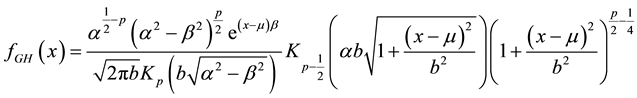(7)

where K_p(z) is a modified Bessel function of the third kind with index p and the five parameters a, b, m, b, p satisfy conditions a> |b|, m, p ÎR, and b > 0.

The GH distribution class is a desirable class for the purpose of risk-neutral distribution approximation because of its salient statistical properties. Most important of all, due to its heavy-tail property which the normal distribution does not possess, GH distribution has many applications in the fields of modeling financial markets and risk management. The GH distribution is also closed under linear transformations. When the first four moments of the risk-neutral distribution are known, there are two subclasses of GH distribution that can be used to compute the risk-neutral distribution: the Normal-inverse Gaussian (NIG) distribution and the VG distribution, since both types of distribution can be completely characterized uniquely by its first four moments. As both NIG and VG distributions appear to be closely connected, and VG has a larger domain of feasibility, we shall employ the VG distribution for modeling the 4-moment risk-neutral distribution in this paper.¹

VG (a, b, m, p) distribution is obtained by keeping a > |b|, mÎR, p > 0 and letting b go to 0 in Equation (7). The parameters can be identified only if. Let, then has unique solution RÎ(0, 1). Denote by M, V, S, K the mean, variance, skewness and excess kurtosis of a VG (a, b, m, p) random variable. In this case we have

.

Note that, in Equation (4), in Equation (5), and

in Equation (6). The condition of C < 1 is called the feasible domain for this probability distribution. In a large percentage of the cases, there would be no violation of this feasibility. For some occasional sample where the skewness S may be too large positively or negatively relative to kurtosis due perhaps to small estimation errors from the BKM procedure, then the computation of the parameters can be carried out by relaxing and increasing K value above the implied kurtosis from the options. From the above, it is seen that the VG risk-neutral distribution can be computed once we obtain an effective set of option prices to infer the risk-neutral moments.

2. New Approach to Density Estimation

In the new approach to estimation of physical densities, we first use current market information obtained from traded options to infer risk-neutral moments of the underlying asset returns over different horizons. For each horizon, the moments are fitted to a general 4-moment Variance Gamma risk-neutral probability distribution of future market prices. We then compute a Radon-Nikodym derivative and its probability distribution, and use this to transform the risk-neutral distribution of the underlying to its physical or empirical distribution.

To place the new approach in context, we provide empirical support by employing intra-day E-mini S&P 500 European-style weekly options data and also the E-mini S&P 500 Futures intra-day data from August 2009 to December 2012 obtained from the Chicago Mercantile Exchange (CME). These options trade actively two weeks before its expiration date. We incorporate all options, including the in-the-money (ITM) options, to capture the information contained in these options. The options data are cleaned by removing a small percentage of prices that violated no-arbitrage bounds. The risk-free rate used in our computation is the yield on the secondary market 4-weeks Treasury bills reported in the Federal Reserve Report H.15.

BKM procedure requires option prices of a continuum of strikes. If option prices are available for all strike prices, then the required integral is straightforward to calculate using any numerical integration method. However, market option quotes are available only for a finite range of discrete strike prices and this will incur a bias in the calculation of risk neutral moments (RNMs) (see Jiang and Tian [11] ).

To tackle the problem caused by these limitations, we consider in-the-money (ITM thereafter) options. We believe that these options do carry information about their underlying and should not be truncated unnecessarily. To incorporate these ITM options, once we apply the data filers, we use the put-call parity equation to transform the ITM options into their respective OTM options. In this way we will be able to increase the number of options in our sample space by including these synthetic OTM options and thereby reducing the bias considerably.

Since the put-call parity equation is also a model-free no-arbitrage formula, by using this transformation, we are able to preserve the information content in these ITM options and at the same time use it to calculate the risk neutral moments (RNM) without imposing any model bias. We extract the RNM for which at least two OTM calls and two OTM puts are in our sample set. We then use the numerical method of piece-wise cubic Hermite interpolation to evaluate the integrals. Piece-wise cubic Hermite interpolation has a local smoothing property, and therefore produces more stable estimates as compared to cubic splines.

The results of extracting these risk-neutral moments are reported below. We show the RNM for the case of a horizon of 1 day. There are a total of 3271 observations in this sample. We average the RNM across the days and report them in Table 1.

Table 1 shows that the risk neutral distributions on average have more negative skewness and much higher kurtosis than that of a normal distribution. The RN moments computed for each day are also highly variable over the period from August 2009 to December 2012.

Assume over a short horizon that the implied risk-neutral rate of change in the futures as obtained from the futures options is nearly equal to the spot index return over the same horizon. The futures price would converge at maturity to the spot index at that time. Suppose S₀ is the current index price or price of a well-diversified S&P 500 portfolio, and S_T is the random price at maturity in horizon T. Let E^Q(×) denote expectation under the risk-neutral measure, and let E^P(×) denote expectation under the empirical or the physical measure. Suppose R is the risk-free rate over horizon T. Let p be the market risk premium or the ex-ante expected rate of return on the market index. Then,

.

Thus,

.

Or,

. (8)

We introduce a random Radon-Nikodym derivative of P-measure with respect to Q-measure X. X can also be written as the ratio of the two densities, i.e.

.

Then from Equation (8),

Table 1. Implied S&P 500 1-day return risk-neutral moments. August 2009-December 2012.

. (9)

X has the property that, and. We model such that

when S_T approaches zero, the empirical density approaches zero much faster than. Given this specification, we develop two equations as follows to solve for and.

,

and

.

We perform the empirical work on the options and risk-neutral moments on various days in December 2012. On 13 December 2012, the RN density function via Equation (7) specialized to the VG case is shown in Figure 1.

The risk-neutral densities found above can be used to obtain by numerical integration the terms,

, and. g₁ and g₂ are then estimated, and can be found. The Radon-Ni-

kodym derivative X is plotted against S_T in Figure 2. Figure 3 shows the estimated density function of X(S_T) under the Q-measure.

From the function X(S_T), we obtain the empirical density function

.

Thus the empirical or physical density function of the 10-day underlying S&P 500 index return can be constructed by linking up Figure 1 and Figure 2, and using a large number of discrete points to produce Figure 4.

Figure 1. Risk-Neutral Density Function of S&P 500 Index. The estimated VG parameters are, , and.

Figure 2. Estimated Radon-Nikodym derivative of P-measure with respect to Q-measure. The estimated parameters are and. The horizontal axis shows the index price S_T.

Figure 3. Estimated Radon-Nikodym derivative PDF.

Figure 4. Empirical probability density functions under Q&P measure.

Figure 5 shows that if we use the usual lognormal distribution assumption on stock index returns (or normality assumption on the log-returns) the tail risk is much lower than that produced by our method via the VG distribution and the transformation to empirical density. In the graph we call this the log VG distribution of index price in the horizon.

3. Application: Computation of VaR

Value-at-Risk (VAR) was a quantile risk measure first used by actuaries before it became adopted as a standard risk measure by regulators (see Jorion [12] ). In 1996, the Basel Committee on Banking Supervision (BCBS) issued an amendment to the 1988 Basel Accord to allow banks to use proprietary in-house models to measure their trading book market risks. The model that has become widely used is the daily VaR measure. For example, if the VaR on a portfolio is $X over one day at 99.9% confidence level, then there is only a 0.1% chance that the portfolio value will drop by at least $X over one day.² Artzner et al. [13] published an influential paper showing that the VaR measure, unlike other measures such as expected shortfall (ES), does not satisfy the sub-addi-tivity property (being part of a coherence framework) which necessitates risk measure reduction under diversification. Since May 2012, the Basel Committee on Banking Supervision (BCBS) has advocated a switch from VaR to the ES measure, and a corresponding adjustment in confidence levels from 99% for VaR to 97.5% for ES. See BCBS [14] [15] .

Figure 5. Empirical probability density functions.

In recent research, Danielsson [16] and Danielsson et al. [17] find that VaR is mostly sub-additive, except for the fattest tails that are quite unlikely except in extreme situations. Yamai and Yoshiba [18] find that it is difficult to back-test the ES method as a very large sample is required. For similar reason, Yamai and Yoshiba [19] also find that ES requires a larger sample size than VaR to provide the same level of accuracy. Kou et al. [20] suggest that coherent measures such as ES may not be as robust to changes in data within a finite sample.

These results point to the lesser stability of ES as a risk measure. The impetus for a switch away from VaR is mostly recognized as the inability of VaR under the usual normality assumption or under historical sampling to produce a large enough loss estimate, something that was seen during the Global Financial Crisis. In any case, VaR is still required to be computed as the conditioning variable for calculating ES. Why VaR typically underestimates market risk is due to wrong specification of the underlying distribution such as normality or log- normality. In this section we employ the new statistical approach to compute VaR with minimal specification error since the inputs we obtain are non-parametrically implied from traded option prices.

In the following tables, we show some comparisons of VaR computed using our approach described in the earlier sections and using the classical log normal distributional assumption. The comparisons are done wth several different days in December 2012 and different horizons to check the robustness of the results. In addition, we want to highlight some useful application this approach would allow us to carry out.

In Table 2, we show that this approached is able to update daily the VaR values of a given day in the future using new information from the options. In Table 3, we show that in a given day this approach is able to project different VaR values for different horizon into the future.

From Table 2 and Table 3, it is clear that the classical lognormal distributional assumption produces VaR estimates that largely understate the tail risk. On the other hand, our method using information from traded option prices produce VaR estimates that are much closer to estimates of expected shortfall. At 99% confidence levels, the log VG method we use produces VaR estimates that are about twice those produced by the classical lognbormal method. Thus, the key issue is not in the use of VaR but rather the appropriate method of estimating it via a more accurate estimation of the physical density.

4. Conclusions

There are key industry applications requiring estimation of physical densities of return distributions. In this paper we show a new statistical approach to estimating physical densities of S&P 500 index futures price distribution. This is done via non-parametric implied moments, fitting with a 4-moment distributional function, and transforming the risk-neutral density to physical density via a Radon-Nikodym derivative transform. The method is applied to the computation of Value-at-Risk (VaR) in risk management.

There have been major changes in the way risk, which is perceived and estimated in the banking and finance industry. The use of VaR has a long history. Although there have been major criticisms of VaR, it appears that its key drawback is in its perceived inability to capture the tail risk of market losses. Although the BCBS has before supported VaR, in recent years, it has switched to advocating using expected shortfall. However, ES is estimated conditional on VaR, giving rise to the possibility that estimation and model risk for ES will be strictly higher

Table 2. Time-series of the computed VaR for 28 December 2012. Note that 24^th December 2012 is left out because the market closed early that day.

Table 3. Computed VaR on 26 December 2012 for different horizons.

than for VaR. Besides, there are studies which point to the instability of ES estimates. ES as well as VaR are both prone to mis-specification errors when there are exogenous assumptions about the underlying distribution such as in the classical lognormality approach. Historical sampling approach on the other hand faces the issue of sampling errors. It is also harder to back-test ES than VaR.

Our key application in this paper shows that VaR can be estimated with minimal specification bias if we use information directly from the traded option prices of the underlying. The novelty of our approach is that it avoids unnecessary mis-specification bias as we do not need to assume a particular empirical distribution of the underlying asset returns. From the option prices we can imply risk-neutral moments with which to fit a very general 4-moment (or 4-parameter) Variance-Gamma (VG) distribution that is popular in finance due to its ability to model heavy tails and skewness.

In practice, different Radon-Nikodym derivative functions can be tested and calibrated to obtain the empirical distribution. As option prices trade frequently, the risk-neutral distribution can be updated frequently for transformation into the empirical distribution. This provides for timely updating of the VaR measures. Our results show that the new density estimation approach is able to yield more accurate of VaR measures in capturing the large tail risks. The new approach is also useful in other risk measures such as conditional value at risk where mis-specification bias in physical distribution can be a major issue.

NOTES

¹We also consider the A-type Gram-Charlier expansions to model 4-parameter distributions, but this approach has the serious drawback that some possible moments may not be able to imply a proper distribution function.

²In market practice, Basel II requires banks to apply 99% confidence level over a horizon of 10 trading days, and the capital charge would be the higher of the previous day’s VaR and a factor, at least 3, times the average of the daily VaR of the preceding 60 trading days. Banks also use other confidence levels and 1-day horizon for measuring VaR for internal control purposes.

Conflicts of Interest

The authors declare no conflicts of interest.

References

[1]	Rubinstein, M. (1996) Implied Binomial Trees. Journal of Finance, 49, 771-818. http://dx.doi.org/10.1111/j.1540-6261.1994.tb00079.x
[2]	Jackwerth, R. and M. Rubinstein (1996) Recovering Probability Distributions from Option Prices. Journal of Finance, 51, 1611-1631. http://dx.doi.org/10.1111/j.1540-6261.1996.tb05219.x
[3]	Breeden, D.T. and Robert H. Litzenberger (1978) Prices of State-Contingent Claims Implicit in Option Prices. The Journal of Business, 51, 621-651. http://dx.doi.org/10.1086/296025
[4]	Longstaff, F.A. (1995) Option Pricing and the Martingale Restriction. Review of Financial Studies, 8, 1091-1124. http://dx.doi.org/10.1093/rfs/8.4.1091
[5]	Chernov, M. and Ghysels, E. (2000) A Study towards a Unified Approach to the Joint Estimation of Objective and Risk Neutral Measures for the Purpose of Options Valuation. Journal of Financial Economics, 56, 407-458. http://dx.doi.org/10.1016/S0304-405X(00)00046-5
[6]	Bakshi G., Kapadia, N. and Madan, D. (2003) Stock Return Characteristics, Skew Laws and the Differential Pricing of Individual Equity Options. Review of Financial Studies, 16, 101-143. http://dx.doi.org/10.1093/rfs/16.1.0101
[7]	Carr, P. and Madan, D. (2001) Optimal Positioning in Derivative Securities. Quantitative Finance, 1, 19-37. http://dx.doi.org/10.1080/713665549
[8]	Barndorff-Nielsen (1977) Exponentially Decreasing Distributions for the Logarithm of Particle Size. Proceedings of the Royal Society of London, 353, 401-419. http://dx.doi.org/10.1098/rspa.1977.0041
[9]	Eberlein, E. and Keller, U. (1995) Hyperbolic Distributions in Finance. Bernoulli, 1, 281-299. http://dx.doi.org/10.2307/3318481
[10]	Eberlein, E. and Hammerstein, E. (2004) Generalized Hyperbolic and Inverse Gaussian Distributions: Limiting Cases and Approximation of Processes. Seminar on Stochastic Analysis, Random Fields, and Applications IV.
[11]	Jiang, G.J. and Tian, Y.S. (2005) The Model-Free Implied Volatility and Its Information Content. Review of Financial Studies, 18, 1305-1342. http://dx.doi.org/10.1093/rfs/hhi027
[12]	Jorion, P. (2000) Value at Risk. 2nd Edition, McGraw-Hill, North-America.
[13]	Artzner, P., Delbaen, F., Eber, J.M. and Heath, D. (1999) Coherent Measures of Risk. Mathematical Finance, 9, 203-228. http://dx.doi.org/10.1111/1467-9965.00068
[14]	Basel Committee on Banking Supervision (2012) Fundamental Review of the Trading Book.
[15]	Basel Committee on Banking Supervision (2013) Fundamental Review of the Trading Book: A Revised Market Risk Framework.
[16]	Danielsson, J. (2013) An Evaluation of Basel III VaR and ES Probabilities. http://www.modelsandrisk.org/basel/
[17]	Danielsson, J., de Vries, C., Jorgensen, B., Mandira, S. and Samorodnitsky, G. (2013) Fat Tails, VaR and Subadditivity. Journal of Econometrics, 172, 283-291. http://dx.doi.org/10.1016/j.jeconom.2012.08.011
[18]	Yasuhiro, Y. and Yoshiba, T. (2002) On the Validity of Value-at-Risk: Comparative Analyses with Expected Shortfall. Monetary and Economic Studies, Bank of Japan.
[19]	Yasuhiro, Y. and Yoshiba, T. (2005) Value-at-Risk versus Expected Shortfall: A Practical Perspective. Journal of Banking and Finance, 29, 997-1015. http://dx.doi.org/10.1016/j.jbankfin.2004.08.010
[20]	Steven, K., Peng, X. and Heyde, C.C. (2013) External Risk Measures and Basel Accords. Mathematics of Operations Research, 38, 393-417. http://dx.doi.org/10.1287/moor.1120.0577