Basic Limit Theorems for Light Traffic Queues & Their Applications ()
1. Introduction
The word queue derives its meaning from the Latin word “cauda” which means tail. Literally, to queue is to wait, of course for a reason which is to receive service. On the other hand, queuing theory is the mathematical study of formation and behavior of queues involving problems connected with traffic congestions and storage systems. This definition extends the relevance of modeling queuing systems to a wide variety of contentious situations for instance, how customers of a service shop checkout lines (arrival process), how lines can be minimized (queuing analysis), how many servers a business person should employ (server capacity), how long a customer waits for service (waiting time analysis) and so on. Generally, the objective of queuing theory is relieving problems in business settings primarily, in operational management and operations research.
In this note, we study business queuing systems with arrival rates less than service rates. This type of queuing system is called light traffic queuing system and is found in businesses such as manufacturing, transportation, shops and telecommunications today. Because the approach here is practical, the note is restricted to those business queues where arrivals occur as Poisson inputs and services are exponential.
Our motivations stemmed from the need to bring Mathematics closer to business in both methodology and application. A large number of business persons believe that Mathematical proofs covering any subject of application are too abstract for real life business transactions and operations. This assertion is evident in one of the many discussions held between ourselves and some petty business persons on how Mathematics will help improve their day to day business transactions. For instance, in a unique discussion session, one business person argues that Mathematics is extremely hard and devoid of practical applications. Similarly, another one argues that translating the difficult results of Mathematics is not an easy task even to students and academics not to talk of a business person who is engaged with day to day selling of commodities. While this believe is strong among business persons, and is valid, it may not necessarily reflect the truth of the situation. It is well known that Mathematics contributes greatly to the advancement of systems and societies through understanding and application of results to various fields of endeavors such as business. However, the achievement of this goal is possible if our results are brought down to a level that is understood by many. In this note, we are motivated to simplify the level of difficulty in an aspect of Mathematics of varied applications in the business field in order that understanding the goodness of Mathematics as it relates to business development will be appreciated. This is for the purpose of achieving business advancement amongst business persons without Mathematical appreciation for better operations and improvements.
The note starts with a brief historical background of queuing theory and some preliminaries required for easy understanding of the Mathematics used here. In Section three, general methodologies leading to some interesting results are discussed. These methods are not new. Similar ones can be found in the literature. Section four provides applications of the general concepts and in Section five; we realize them through relevant Examples. Here, instances covering several aspects of business transactions are considered. The note is concluded in Section six with summaries.
2. Historical Background
From evolutionary perspective, Medhi [1] dated the origin of queuing modeling as far back as 1909 when the Danish Mathematician Agner Krarup Erlang published his fundamental paper on congestion in telephone traffic. Erlang, in addition to formulating analytic practical problems and solutions, laid a solid foundation to queuing system modeling in terms of enacting basic assumptions and techniques of analysis. Interestingly to date, we are using them even in the wider areas of modern communications and computer systems. For instance, using Erlang basic assumptions and techniques, Ericsson telecom developed a programming language called Erlang used in programming concurrent processes and verifications such as the conditional term rewriting systems (CTRS). His works led to the development of queuing models vital for analyzing lost and delay in operation systems (similar to that of the M/M/C discussed here.). The first model is called the Erlang-B and is used to compute probability that, an incoming arrival is rejected. Similarly, the Erlang-C model gives the probability that an arrival has to wait before service.
Though, Erlang pioneered Mathematical modeling in queuing systems especially its applications to operations research, the pioneer of modeling from the perspective of stochastic process was Kendal. In 1951, Kendal developed and introduced certain notations which to date are adopted to denote queuing systems. The Kendal’s A/B/C notation specifies three basic characteristics in a given queuing system namely; the arrival process (A), the service distribution (B) and the number of servers in a system (C). Similarly, Kendal’s integral model relating the Laplace-Stieljes transformations of the busy period and that of the arrival process is a remarkable achievement and breakthrough in the field of queuing modeling. To date, lots of priority models covering peak and rush hour (steady state models) service distributions are computed using the model and several numerical models to analyze it have been developed. The Kendal’s era in queuing studies marked the beginning of mathematical modeling of queuing processes as stochastic processes.
After these breakthroughs, modeling trends shifted from conditioning and design to rigorous applications in form of averages and other statistics of operational significance. A good Example is the work of D.C. Little. In 1961, Little came up with a model relating the averages of three quantities in every queuing system in what is known in the queuing parlance as little’s formula. The formula relates the average number of customers in the system or in the queue to the average sojourn or waiting times. To date, the model is applied in analyzing expectations in light traffic queues (similar to the ones discussed here) in manufacturing and other service systems as well as in decision making to quantify expectations of parameters for better service delivery. The Erlang- Kendal-Little’s models (EKL models) are the initiating models in queuing studies.
After this era, a lot of sub areas of interest continue to emerge especially in the 40’s. For instance, Franken et al. [2] indicated that in the early 50’s, Mathematicians were faced with the onerous challenge of developing appropriate Mathematical tools to describe sequence of arrivals in a given system. The first stage of this development was taken by Conny Palm in 1943 and was made Mathematically precise and well expanded by Aleksandr Khinchine. In 1955 precisely, Khinchine studied point processes on the positive real line which he addressed as stream of homogenous events. This development opened further examination of similar areas among others including that of insensitivity of queuing systems. Here, existence and continuity statements (stability conditions for a model) and relationships between time and customer stationery quantities with special inputs were emphasized. This led to the emergence of a new class of random processes connected with point processes which seemed most suitable for describing queuing systems. The new class is termed random processes with embedded Marked Point Process (PMP)1. The development of this class of process was attributed to Khinchine and Kendal in 1976 and was the base for modeling in every sense of the word, as far as modeling light traffic queuing systems is concerned.
The last four decades to date symbolizes an era of model development2 as Medhi [1] implies. Queuing theorists today seemed more interested in model developments, applications and extensions. This era is of modeling and lots of queuing systems were modeled and developed. What we witnessed of late is a shift in paradigm that centers on creating models to capture every bit of system development, advancement and conjecture. Models may be classified under two categories; deterministic models (stable models such as the case here) and stochastic models. The methodology today is to pose a problem and model it in transient or limiting sense (Here, our analysis is purely a limiting case analysis). However, it requires the mathematical analysis of existence of solution so that the constructed model is realistic. The central limit theorem and the maximum principle form the basis for proofing existence of queuing models today.
Limit theorems over the years such as the ones used in this note, have been developed for various queuing models to show limiting behavior. For instance, on light traffic models, the series of deterministic results obtained over the years on these models are enormous. Federgruen & Tijms [3] obtained the stationery distribution of the queue length for the M/G/1. Hoksad [4] and Hoksad [5] worked on a more general queue called the M/G/m in terms of its limiting state solution and its specific case. Smith [6] specified the system performance of a finite capacity queue called the M/G/C/K. Also, Tijms et al. [7] approximated the steady state probabilities for the M/G/C queue. For the classical M/G/1 queue with two priority classes under preemptive and non-preemptive- resume disciplines, Abate & Whitt [8] derived these limit theorems. They proved that the low-priority limiting waiting-time is a geometric random sum of independent and identically distributed random variables like the M/G/1 first come first served waiting-time distribution. Similarly, the asymptotic behavior of tail probabilities is such that there is routinely a region where these probabilities have non-exponential asymptotics even if the service time distributions are exponential. In addition, the asymptotic formed tends to be determined by the non- exponential asymptotics for the high-priority busy-period distribution etc.
Finally, light traffic modeling is near complete today and modeling is basically given application outlook for better system performance and evaluation.
3. Preliminaries
3.1. The M/M/C Model
By the M/M/C queuing model3, we refer to all service stations where customers arrive according to a Poisson process independently with a mean arrival rate of λ, then receive service in a time that is exponentially distributed on any of the C servers available in the system.
The number of servers C specifies the type of the M/M/C queue. For Instance, if C = 1 or infinite then, the corresponding queuing model is called the M/M/1 or the M/M/∞ respectively. Researches in this area have shown that in steady state, the M/M/C model is a continuous-time birth-death process.
3.2. Occupation Rate
The occupation rate of a server is the fraction of time the server is busy.
It is the ratio of the arrival rate to the service rate of customers in the system. Denoted normally by ρ, the occupation rate provides information on the stability and class of a queuing system. For instance, if ρ < 1 then, a queuing system is a stable light traffic system otherwise, it is a heavy traffic queuing system.
3.3. Queuing Schedule
This is the ordering principle of a queuing system. It is the rule describing the manner in which customers access the server for service purposes.
A queuing schedule may be First-Come-First-Served (FCFS), a Last-Come-First-Served (LCFS), processor sharing (ps) or priority discipline (pd) etc.
3.4. Poisson Distribution
A random variable W with parameter λ denoting the mean number of arrivals in a fixed interval of time say [0,T] is said to be Poisson if its probability density function is given by

The Poisson distribution is commonly used in queuing modeling to capture inter-arrival times of customers because of thememory-less property therein. This makes it unique and suitable for depicting the realities of arrivals or departures in physical systems such as the telephone and similar traffic systems4.
3.5. Exponential Distribution
A random variable W with parameter μ denoting the mean number of departures in a queuing system is exponential in distribution if its probability density function is given by

Similarly, the exponential distribution is used in modeling light tail distributions such as the service process in a queuing system of shops, telephone centers etc.
3.6. Erlang Distribution
A random variable W with a mean w/μ is said to have an Erlang-w  distribution if it is a sum of w-independent random variables each exponentially distributed.
Basic Limit Theorems:
Theorem 3.1: The limiting probability distribution for a general birth-death process in a state say k is given by
 (1)
(1)
where  and
and  are the individual birth and death rates and p0 is the probability that the generating process is in the idle state.
In steady state5, a birth-death process is time independent almost surely. Thus, if it is generated by a unit service point then, its continuous-time distribution is strictly that of the M/M/1 queue.
Theorem 3.2: Denote by  the stationary customer distribution of a shop queue with a Poisson arrival process and exponential service times operating under the FCFS queue schedule. If
  is the occupation rate of the server then,
  is given by the geometric distribution
 (2)
(2)
The performance measures such as the mean and variance of the model can be computed. We will demonstrate this subsequently.
Now, if the single server here, is replaced by a general value say C where C > 1 then, a new model called the M/M/C queue analogous to a multi-server service system with Poisson arrival rate and exponential service rate is obtained. The parameter for this model is the size of ρ. If ρ is less than unity that is, under light traffic then, steady state could be attained.
Theorem 3.3: For the M/M/C queuing system under light traffic and FCFS service schedule, the stationary customer distribution  is given by
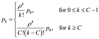 (3)
(3)
In this case,  gives the probability that the system is idle.
The two limiting distributions for the M/M/C model in (3) above give the stationary distribution for the Erlang-B and Erlang-C models6 respectively. The first model gives the blocking probability that a customer is lost by the system and the second model gives the probability that an arriving customer has to wait before being served. There are other relevant cases of the M/M/C queuing model. Of immense importance is the case when the waiting space is bounded. This model is applied in dimensioning service points for instance, a parking lot, a lift etc. In this case, the stationery customer distribution is a slight modification of the above mentioned distributions represented in (3).
Theorem 3.4:
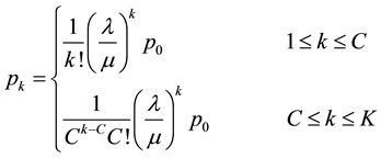
For the M/M/C/K queuing model with finite waiting capacity K, let  be the steady state customer distribution and ρ, the occupation rate of the C-servers in the system. Under the FCFS schedule, the two-case stationery customer distribution
  is given by
 (4)
(4)
and ![]() is the idle state distribution given by
is the idle state distribution given by
![]() (5)
(5)
Here, A7 is the ratio λ/μ where λ is the average arrival rate of customers in the system and μ is the average service rate of a single exponential server in the system. A basic assumption here is that the service rate of all the C- servers is assumed approximately equal.
Theorem 3.5: Suppose that a FCFS-M/M/1/K queuing system is given, where K is the capacity of the system. If ρ is the occupation rate of the server, then the light traffic model for the steady state customer distribution ![]() is given by
is given by
![]() (6)
(6)
where ![]() is given by
is given by
![]() (7)
(7)
The stability condition for this model is that the server occupation rate ρ = 1. If ρ is less than one, the model reverts to the M/M/1 infinite capacity queue.
Similarly, there are real life scenarios where priorities8 are observed9. If priorities are observed then, the model is pre-emptive. In this case, the customer with the highest priority is serviced even when the low priority customer is receiving service.
Theorem 3.6: In an M/M/1 queuing system with priority customers say type 1 and type 2. Let ρ1 and ρ2 denotes the occupation rates for both customer classes respectively. Under the pre-emptive priority scheduling, the stationery customer distribution for type 1 customers is given by the geometric distribution
![]() (8)
(8)
For the type 2 customers, it is a little bit tricky and we ignore it completely.
Suppose, we wish to model the distribution of customers in a river with Poisson arrival process and exponential service times. In this case, we are talking of a model whose server size is infinite. The model is depicted as the M/M/∞and is applied in modeling completely open-server queuing systems.
Theorem 3.7: For the M/M/∞ queuing model with occupation rate ρ and FCFS service schedule, the stationery customer distribution is given by
![]() (9)
(9)
Theorem 3.8: Suppose ![]() is the stationery waiting time of an arbitrary customer where each Si denotes the waiting time of a customer ahead of the arbitrary customer and Si is exponential at a rate μ. If N is geometric with zero idle state then, the stationery waiting time distribution of customers in the M/M/1 queuing model having λ as a mean arrival rate and μ as mean service rate is the light tailed10 exponential distribution
is the stationery waiting time of an arbitrary customer where each Si denotes the waiting time of a customer ahead of the arbitrary customer and Si is exponential at a rate μ. If N is geometric with zero idle state then, the stationery waiting time distribution of customers in the M/M/1 queuing model having λ as a mean arrival rate and μ as mean service rate is the light tailed10 exponential distribution
![]() (10)
(10)
In this case also, ρ denotes the server occupation rate. Similarly, the response time distribution which measures the total time a customer stays in the system including his service time has a cumulative distribution.
Theorem 3.9: Under the condition of theorem 2.8 above, the cumulative distribution of the response time T for the FCFS-M/M/1 queuing system is the exponential distribution
![]() (11)
(11)
Similarly, for the M/M/C model, the response time distribution exists.
Theorem 3.10: For the FCFS-M/M/C model with finitely many servers C, given that, the stationery mean arrival and service rates are λ and μ respectively, then the complementary waiting time distribution is light tailed exponential and is given by
![]() (12)
(12)
In this case, ![]() is the service distribution of all waiting customers in the system.
is the service distribution of all waiting customers in the system.
4. Analytic Applications
Example 4.1:
Suppose we wish to inquire on what to expect in a call center where customers arrive according to a Poisson process at a rate say λ to make calls with service times similarly exponentially distributed at a rate say μ when the arrival rate is strictly less than the service rate. Obviously, we are in the M/M/1 environment and performance measures such as the expected number of customers E[N], expected response time E[T], expected queue length E[Nq] and expected waiting time E[W] can be computed analytically.
Solution 4.1:
From elementary probability, we have
![]() (13)
(13)
That means by (2)
![]() (14)
(14)
Similarly, the expected response time for the call center can be analyzed. The following theorem due to D.C. Little is significant in analyzing this parameter.
Little’s Theorem
Under steady state condition, the average number of customers E[N] in a system is a product of the average at which customers arrive λ and the average time E[T] customers spend in the system. In mathematical sense,
![]() (15)
(15)
Thus, if we apply (14) on the expected number of customers E[N], the expected response time in the call center E[T] is given by
![]() (16)
(16)
Also, the expectation of the waiting time E[W] can be computed from that of the response time given that, the expected service distribution is known. Define
![]() (17)
(17)
Here, E[S]11 is the limiting expectation that, the call device is busy. This expectation equals to ρ. Consequently,
![]() (18)
(18)
Finally, the number of customers in the queue waiting to make a call can be computed via Little’s theorem connecting the expected number in the queue and the expected waiting time. Thus,
![]() (19)
(19)
Example 4.2:
A telephone business center12 with a single telephone head has two types of customers; customers with urgent call needs (A) and those with normal call needs (B). As a rule, the center gives priority to A over B. Given that, both A and B arrive according to a Poisson process with steady rates λ1 and λ2 respectively and that, the service times of both customer classes is exponentially distributed with a constant mean 1/μ, what is the expected number of customers E[N] in the system and the expected response time E[T] when the priority is preemptive and non-preemptive.
Solution 4.2:
Suppose that![]() . If this condition holds then, analysis is possible.
. If this condition holds then, analysis is possible.
Now, denote by N1 and N2 the number of type A and B customers in the telephone call center respectively. Let T1 and T2 be the respective response times for the two types of customers. Intuitively, the response time of A is independent of B. Thus, for type A customers, we have
![]() (20)
(20)
Similarly, the expected number of customers in the system is equal to
![]() (21)
(21)
For customer type B, we claim that, the service distribution of all types of customers is exponential. Consequently, the distribution of customers in the system will not depend on the service arrangement and so, the joint expected number of customers E[N1 + N2] in the telephone center is given by
![]() (22)
(22)
Furthermore, the expected number of type B customers E[N2] is the difference between the joint expectation (22) and that of the first category. Thus,
![]() (23)
(23)
Finally, under pre-emptive priority the expected response time E[T] is given by
![]() (24)
(24)
Example 4.3
A manufacturing system has finitely many servers C. If customers arrive according to a Poisson process at a stationery rate say λ and are served negative exponentially on the average 2/μi. What is the expected queue length13 and the expected waiting time in the system.
Solution 4.3
Let ![]() be the expected number of customers who upon arrival, has to waiting before service and E[W] be their expected waiting time in the system. We can extract for instance the limiting distribution of
be the expected number of customers who upon arrival, has to waiting before service and E[W] be their expected waiting time in the system. We can extract for instance the limiting distribution of ![]() from the distribution given in (3). The extraction process will give
from the distribution given in (3). The extraction process will give
![]() (25)
(25)
where ![]() is as defined in (3). After substitution and rearranging, we will have
is as defined in (3). After substitution and rearranging, we will have
![]() (26)
(26)
Thus, the expected waiting customers is given by
![]() (27)
(27)
And by dividing (26) by the arrival rate λ, the expected waiting time of customers in the system follows. This is consequence of Little’s theorem. Thus,
![]() (28)
(28)
Similarly, that of the number of customers and the response time can also be computed. We left it to the reader as an exercise!!
Example 4.4
In a certain river, customers arrival follow a Poisson process at a rate of λ to take service with service times exponentially distributed at a rate of μ. What is the expected number of customers E[N] in the system and the mean response time E[T].
Solution 4.4
Since it is unimaginable to comprehend a lost customer in a river, we can model it as an M/M/∞. Similarly, it can be idealized that the mean number of services is the same as the sum of all small portions of the river being put to use out of its area14.
Now, remember that for the M/M/∞, the limiting distribution is a Poisson distribution with parameter ρ. Consequently, E[N] is the mean of a Poisson random variable. In this case, E[N] is simple the server occupation ρ. Similarly, the other expectation can be seen in the light of Little’s theorem.
5. Realistic Applications
Example 5.1
A local council wishes to determine the size and staffing of a local maternity hospital. Historically, it was gathered that, there is the average of 10 births per day in the ward to which most women are discharged after 2 days from the ward. Though, in one year, about 5 percent of the women admitted take 10 days for different complications. What is the average length of stay in the ward15.
Solution 5.1
Here, the council is interested at how long a given admit will stay, possibly for reconstruction and re-staffing. In this case, Little’s theorem provides the solution.
Now, denote by E[L] the expected length of stay of admits in the ward. Intuitively, this period depends on the type of admit. If we let λ1 and λ2 to represent the arrival rate of admit type 1 and admit type 2 respectively corresponding to the response times T1 and T2 then by Little’s theorem, we have
![]()
Example 5.2
A telecom company wishes to upgrade her system capacity. On records, calls arrive in the existing system at a rate of 500 per minutes and each call resides for an average of 5 minutes. If the system presently has 20 service points, what is the stationery distribution of lost calls in this system.
Solution 5.2
In telecommunications modeling, the server occupation rate is commonly known as the average system load. Since, the interest here is on lost customers, the Erlang-B model is most suitable in this computation. Consequently, using
![]() (29)
(29)
Where C is the number of servers and A is the average system load, we have16
![]()
Example 5.3
The department of Mathematics of a University X has a single printer connected to the local area network (LAN) of the department. Recently, it is observed that, the delay time of processing printing jobs is on the increase and there is the need to reduce it. Show by analytic modeling how this problem can be tackled out.
Solution 5.3
This is a decision making problem. Suppose printing jobs arrive the printer as Poisson process independently at a rate of λ and are served exponentially at a rate μ1by the problematic printer. There are 2 possible ways to solve this delay problem:
1) A new printer with service rate aμ1 where a > 1 will be bought to replace the existing printer.
Under this modeling, let E[T1] and E[T2] are the expected response time of the existing and the new printer respectively. Then, it is clear for this M/M/1 model that,
![]()
Thus,
![]()
2) If the department is in no income state then, n-old printers17 (n > 1) similar to the existing one be put to usage side by side with the existing printer.
Under this modeling, the arrival rate for the M/M/C queuing system here is partitioned to be on average, λ/n. Let E[T] denotes the expected response time of the printing arrangement. Obviously,
![]()
Example 5.4
An M/G/2 queuing system has one-exponential and one general server. Given that, the general server is regularly varying at infinity index ![]() and the system is conditioned such that, the general server is available for use only if the exponential server is busy, what is the steady state expectation of the number of customer in the system. Also, Compute the expected response time E[T] if the arrival rate is 0.5μ, where μ is the exponential service rate.
and the system is conditioned such that, the general server is available for use only if the exponential server is busy, what is the steady state expectation of the number of customer in the system. Also, Compute the expected response time E[T] if the arrival rate is 0.5μ, where μ is the exponential service rate.
Solution 5.4
Denote by B(t) the service time distribution of customers served by the regularly varying server with a mean of β. If the arrival and the exponential service rates are λ and μ respectively then, in steady state, the stability condition for this system is λ < μ + 1/β holds. Under this condition, we can argue that if λ < μ + 1/β, it is trivial that is λ < μ. This is analogous to keeping a customer with an infinite service time on the regularly varying server. Consequently, the M/G/2 model in this case behaves like the M/M/1. Thus, the limiting expectation for the number of customers in the system is given by (20). Now, given that, ρ = 0.5 and E[T] is the expected response time, it is obvious that, E[T] = 2/μ .
Example 5.5
A bank has 13 counters. Customers arrive as a Poisson process at a rate of 3 per minute and stay in a single queue. If each counter staff needs on average 4 minutes to deal with a customer. What is the steady state probability that all the counter staff are idle.
Solution 5.5
We can easily compute this distribution if we model the bank as an M/M/C queue. In this case, C = 13, λ = 3, μ = 1/4, λ/μ = 12 and ρ = λ/C μ = 12/13. Applying the idle probability distribution for the M/M/C model given by
![]() (30)
(30)
We have
![]()
Exercises:
1) In a gas station with a single pump, cars arrive according to a Poisson process at an average of 20 cars per hour to receive service. The time required for service is exponential at a mean rate of 3 minutes. Given that, a car may refuse to enter the station with probability qn = n/4, determine;
a) The stationary distribution of cars in the station.
b) The mean number of cars at the station.
c) The mean response time of cars remaining in the station.
2) A repair man fixes broken computers. The repair time is deemed exponentially distributed with a mean of 30 minutes. Broken computers arrive at his repair shop according to a Poisson stream with an average of 10 broken computers per day (he works for 8 hours in a day).
a) What is the fraction of time that the repair man has no work to do?
b) How many computers are on average, at his repair shop?
c) What is the mean response time for a computer to be repaired?
3) Consider two parallel machines A and B having a common buffer where jobs arrive according to a Poisson process with rate β. The processing times (service times) are exponentially distributed with means 1/μ1 for A and 1/μ2 for B, where (μ2 < μ1). The service discipline is first come first serve and during idle state, an arrival
is assigned the faster machine. Assuming that, ![]() , determine;
, determine;
a) Determine the distribution of the number of jobs in the system.
b) Use this information to derive the mean number of jobs in the system.
c) Decide when it is better not to use the slower machine at all.
4) A computer consists of 3 processors. Their main task is to execute jobs from users. These jobs arrive according to a Poisson process with rate 15 jobs per minute. The execution time18 is exponentially distributed with mean of 10 seconds. Given that, when a processor completes a job and there are no other jobs waiting to be executed, the processor starts to execute continuous-time maintenance jobs that are exponentially distributed with a mean of 5 seconds. But as soon as a main job arrives, the processor interrupts the execution of the maintenance job and starts to execute the main job. The execution of the maintenance job will be resumed later (at the point where it was interrupted).
a) What is the expected number of processors busy with executing jobs from users.
b) How many maintenance jobs are on average completed per minute.
c) What is the probability that a job from a user has to wait.
d) Determine the mean waiting time of a job from a user.
6. Conclusion
We demonstrate modeling in light traffic queuing systems for business owners with little appreciation for Mathematics. The aim is to encourage the use of the well grounded theories of the subject to areas where application will lead to improvements and better service provision. The functional limit theorems selected and applied here are some of the well known theorems in queuing theory. As for the proofs and more general discussions on this subject, there are vast amount of literature covering this topic on queuing theory today.
Acknowledgements
We are grateful to all the literature sources used in this note. Also is to the anonymous referees.
NOTES
*Corresponding author.
![]()
1A special case of the PMP is a piece wise Markov process.
2Quantum of light traffic and heavy traffic models has been formulated and is still on-going.
3First M means Markovian; second M means Exponential and C means number of servers.
![]()
4Though, the Poisson controversy in the internet and communications modeling depicting Poisson based models as obsolete exist today; see [9] , recent researches for instance, [10] have shown that, the observed long-range dependence in the internet traffic does not make the Poisson based models obsolete.
5A state when arrival rate equals to service rate in a given system.
![]()
6These models are to date, relevant in light traffic modeling.
7The parameter A provides information on a unit-server rate of service.
![]()
8Priorities arise normally owing to variations in wants, needs etc of customers. Consequently, it is significant to understand modeling in this sphere.
9Priorities are embedded in our nature. Thus modeling must take account of it for effectiveness of approximations.
10Its convergence is faster. Thus it attains it limit within a realistic service time.
![]()
11This expectation is non-zero for a system in state.
12This type of problems forms the essence of modeling under light traffic in queuing systems. In addition, they are the initiating problems in modeling queuing systems generally.
![]()
13That is, the number of customers in the waiting.
![]()
14With good modeling practice and estimation, the problem could similarly be modeled as the M/M/C/C queuing system. A student of modeling may wish to compute that and compare the two results.
15Problems like this and many others prove the justifications of modeling in the light of social and economic systems for effective management.
![]()
16The student is expected to complete this as a free lunch.
17This may hold only if the existing printer is not the first to be used in the department. Otherwise, the first option suffices.
![]()
18Execution time here means the service time.