Existence and Smoothness of Solution of Navier-Stokes Equation on R³

Ognjen Vukovic^*

Department for Finance, University of Liechtenstein, Vaduz, Liechtenstein.

DOI: 10.4236/ijmnta.2015.42008                

Abstract

Navier-Stokes equation has for a long time been considered as one of the greatest unsolved problems in three and more dimensions. This paper proposes a solution to the aforementioned equation on R³. It introduces results from the previous literature and it proves the existence and uniqueness of smooth solution. Firstly, the concept of turbulent solution is defined. It is proved that turbulent solutions become strong solutions after some time in Navier-Stokes set of equations. However, in order to define the turbulent solution, the decay or blow-up time of solution must be examined. Differential inequality is defined and it is proved that solution of Navier-Stokes equation exists in a finite time although it exhibits blow-up solutions. The equation is introduced that establishes the distance between the strong solutions of Navier-Stokes equation and heat equation. As it is demonstrated, as the time goes to infinity, the distance decreases to zero and the solution of heat equation is identical to the solution of N-S equation. As the solution of heat equation is defined in the heat-sphere, after its analysis, it is proved that as the time goes to infinity, solution converges to the stationary state. The solution has a finite τ time and it exists when τ → ∞ that implies that it exists and it is periodic. The aforementioned statement proves the existence and smoothness of solution of Navier-Stokes equation on R³ and represents a major breakthrough in fluid dynamics and turbulence analysis.

Keywords

Navier-Stokes Equation, Millennium Problem, Nonlinear Dynamics, Fluid, Physics

1. Introduction

In this paper, the following form of Navier-Stokes equations in R³ is studied:

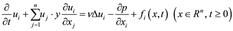(1)

(2)

With initial conditions

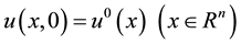(3)

Here, (divergence-free vector field on), are the components of a given, externally

applied force, v is a positive coefficient (the viscosity) and is the Laplacian in space variables. If

Euler equations are considered, then the same set of equation must be applied with the condition that viscosity is equal to zero.

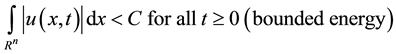
The following conditions must be satisfied as it is wanted to make sure that does not grow large as:

(4)

And

(5)

The accepted solution of N-S is physically reasonable if it only satisfies:

(6)

And

(7)

At the same time, it is possible to look at spatially periodic solutions. We can assume the following conditions:

(8)

Under the condition that is unit vector in. It must be assumed that is smooth and that

(9)

The solution is then accepted if it satisfies:

(10)

And

The problem is to find and analyze whether a strong, physically reasonable solution exists for the Navier- Stokes equation.

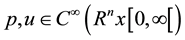
The statement that will be proved is existence and smoothness of Navier-Stokes solutions on R³. Take v > 0 and n = 3. Let be any smooth, divergence-free vector field satisfying (1.4). Take to be identically zero. Then there exist smooth functions, on R³ x[0, ∞] and the above conditions and equations are satisfied.

2. Results

Firstly, the definition of turbulent solutions (Oliver and Titti) [1] is provided. We must define the set of all real vector functions with compact support in such that. We define as the closure of with respect to L^r norm; is the inner product in L². L^r stands for the usual L^r-space over Rⁿ,

. is the closure of with respect to the norm where.

When X is a Banach space, denotes the norm on X. and are the Banach spaces, where and and are real numbers such that. C denotes various constants.

Def 1. (Oliver and Titti) [1] A turbulent solution of Navier-Stokes equation is defined as following:

1) (11)

The relation

2) (12)

Holds for almost all T and all such that

Strong energy inequality

3) (13)

Holds for almost all including, and all.

It is necessary to introduce the Stokes operator in. The following Helmholtz decomposition is obtained:

where. denotes the projection from onto. defines the Stokes operator with domain. A denotes the Stokes operator. denotes the spectral decomposition of self-adjoint operator A.

The existence of turbulent solutions for n = 3 and n = 4 is given by Leray and Kato. In order to derive the next results, theorem from Takahiro Okabe will be introduced.

Theorem 1. Let and let and be

For,

For

Suppose that for for and. If

for some then for every turbulent solution there exist and such that:

(14)

holds for all and for all

Def 2. Let,. A measurable function u defined on is called a global strong solution of Navier-Stokes equation if:

(15)

and u satisfies:

(16)

where denotes the projection from onto of the product of the divergence of solution u and the solution itself.

Takahiro Okabe [2] , in his paper named “Asymptotic energy concentration in the phase of the weak solutions to the Navier-Stokes equation”, proves that turbulent solutions of Navier-Stokes equation become strong solutions after some definite time. So for the turbulent solution of of Navier-Stokes equation there exists such that is a strong solution of Navier-Stokes equation on, then the energy identity exists:

(17)

For. For any fixed, the second term in (16) is estimated from below as:

(18)

From (16) to (18), the following is obtained:

(19)

Afted dividing the both sides of (19) by, the following is obtained:

(20)

By (17), the following is obtained it follows from (17) to (20) that:

(21)

By introducing the new theorem that is proved in Takahiro Okabe’s paper [2] , the following is obtained.

Theorem 2. Let. Let r and m be as

1)

2)

If, every turbulent solution of of Navier-Stokes equation satisfies:

(22)

As.

The following theorem can be proved by using well-known Leray’s structure theorem, every turbulent solution of N-S becomes the strong solution after some time. Although Kato proves that the strong solution decays in the same way as the Stokes flow, we apply different approach by using Oliver and Titti’s paper [1] named “Remark on the Rate of Decay of Higher Order Derivatives for solution to the Navier-Stokes equation”.

By introducing the above mentioned theorem, the following result is obtained and it proves Theorem 1.

This result proves that energy of the molecules of fluid moving is smaller than some value determined by C, n, r, m and it proves asymptotic energy concentration. In order to prove that turbulent solutions are at the same time strong solutions, blow-up time of solutions must be analyzed.

It is demonstrated that Navier-Stokes equation enter some class as it was already proved in arbitrarily short time. Foias and Temam have proved the following solution in the case of periodic boundary condition and for the case of the Navier-Stokes equation on the two-dimensional. Kukavica and Grujic have obtained the given results in spaces. The following lemma must be introduced and it is proved in Oliver and Titi’s paper [1] :

Theorem 3. Let, and. Then there exists a constant such that any two functions v and w in satisfy the inequality:

(23)

The theorem is proved by using Plancherel theorem, the triangle inequality, the inequality

and the convolution estimate. These are the tools used to prove the aforementioned theorem. For further details, look at the aforementioned paper. This theorem demonstrates that the blow-up time is infinite so that the solution is existent. In order to find a solution, it must be captured in some sort of space where the function oscillates. In order to introduce the following solution, a few more results will be introduced.

Firstly, we assume the existence of solutions is known for some T > 0. In order to simplify the notation, the following is set:

(24)

(25)

where is to be specified later.

Then the Gevrey norm is used to find the following result:

(26)

The contribution of pressure term is zero because A commutes with the Leray projection onto divergence free vector fields. Note that:

(27)

By using Theorem 3 and Cauchy-Schwarz inequality, the following result is obtained.

(28)

In order to proceed, we introduce the Theorem 4.

Theorem 4. For all nonnegative p, q and τ we have the following:

(29)

The proof is similar to that in Theorem 3, just it should be noted that for every, one has since on and for.

After introducing the theorem and interpolating by using Theorem 3 and Theorem 4 with, , the similar thing is done with. If we apply the Young inequality, the following result is obtained.

(30)

where. After setting, after interpolating the first term on (26) then use the estimate on (30), the following equation is obtained:

(31)

This proves that there exists a such that is finite for. This proves that if space is finite, then Garvey space is finite which demonstrates the existence of stationary solution.

Now the result of differential inequality for longer time will be derived. The radius of uniform analyticity increases like as as the solutions for heat equation. First the optimal decay rate for Gevrey norm is established, the optimal decay rates for norms of finite order derivatives will be established and it will be extended to infinite order.

If first two terms of Equation (26) are considered and it is assumed that only contribution from linear terms is included, interpolation can be used as well as Young inequality while breaking the second term in several fractions. Theorem 3 provides the following:

(32)

we all together obtain:

(33)

New theorem is introduced, it is already proved by using Plancherel theorem:

Theorem 5. Provided that and, the following is obtained:

(34)

Combining Theorem 5 with and the Young inequality, the following is obtained.

(35)

If we set where and. The following is immediately found.

(36)

So that the first two terms on the right of equation (33) are nonpositive and can be neglected. The main task is now to analyze the nonlinear terms and if possible prove that these nonlinear solutions do not affect the decay properties of the solution to infinite order. Applying the estimate on nonlinear term and by interpolating by using theorem,; is interpolated in an analogous manner. By application of Young inequality, the following is found.

(37)

3. Theoretical Findings

The following differential inequality is obtained.

(38)

As we are considering global asymptotics and blow-up profiles, they are only possible in the presence of a critical controlled quantity or the combination of a subcritical and a supercritical controlled quantity. It turns out that the Navier-Stokes equation according to differential inequality tends to contract these quantities, in that way leading to a useful way to force finite time blow-up. The idea of using minimal surface area as controlled quantities originates from Hamilton. In order to discuss the blow-up time, we introduce the following well known proposition:

Assume that is non-trivial. Let be any immersed sphere not homotopic to a point.

Each such sphere has an energy using the metric at time t. If we define to be

the infimum of over all such. It turns out from standard Sacks-Uhlenbeck minimal surface theory that this infimum is actually attained. The differential inequality is obtained using structure of minimal surfaces and the Gauss-Bonnet formula [3] :

(39)

where is the Ricci scalar. It demonstrates that the change of infimum of energy becomes negative in finite which is absurd. Therefore this forces blow-up in finite time. This means that the solution blows up in a finite time, which is why the surgery approach will be used.

If the above mentioned state holds, then the differential inequality, in order to make nonlinear terms of lower order, has to satisfy the following form:

(40)

where is fixed. First it must be noted that is an increasing function of, so that at the beginning at the initial time, is bounded between when and when. Thus the left side of equation (39) diverges faster than the right side as, so that we can satisfy condition at by choosing small enough. However, what happens when doesn’t converge to 0. Imagine, then the left part of equation is 0 and the right part is higher than zero, but that is not possible, because it is proved above that the infimum of energy becomes negative, that is absurd. So the solution must blow up in some definite and the equation must hold even for as a solution. This proves that the solution is existent and smooth. In order to proceed, we will analyze the nonlinear terms. After having proved that the above equation must hold even for some that does not converge to 0, the only equation that must be solved is the following:

(41)

where. According to assumption that there exist positive real numbers and which may de-

pend on such that for all where is a solution to the Navier-Stokes equa-

tion provided and, where and, a final form of differential inequality is obtained.

(42)

The integrating factor for linear differential inequality is:

(43)

So the following is obtained.

(44)

If we fix small enough so that, the following is concluded:

(45)

If the condition (39) is satisfied for all t, estimate (44) will be global in time. It is sufficient to show the following:

(46)

for some non-increasing function. Estimate (44) shows that this is the case whenever and

(47)

which satisfies the above mentioned conditions and it proves the existence of a solution. As, converges to zero therefore the solution is existent at the beginning, and if the equations exist, then the solution exists in the time.

It is obtained that:

(48)

The upper bound of decay is calculated and given below:

(49)

where is given above according to the following definition and maximum is attained at so the following definition demonstrates:

(50)

(51)

This proves that solution is existent even when does not converge to 0.

Now in order to proceed and analyze the blow-up time, v as the solution of the heat equation will be introduced. It should be proved that the solution between Navier-Stokes and heat solution in can be made sufficiently small so that u must decay at the same rate.

First an estimate on the difference w in. Clearly, it satisfies the following equation:

(52)

(53)

As the heat equation preserves the divergence condition, the following equation is obtained for all. Setting:

(54)

(55)

And repeating the steps, the following result is obtained:

(56)

The second of nonlinear terms arises from (47) by using and choosing the smallest possible. For, the following is obtained:

(57)

The following differential inequality is obtained:

(58)

And the following is obtained:

(59)

After having proved that solution for exists and if we examine the equation, as the distance between heat equation solution and Navier-Stokes equation demonstrates convergence and if the following heat equation solution is found then the solution for Navier-Stokes equations exist and is in the same range as heat equation solution.

Now the heat solution equation Cannon [4] is analyzed. The solution of heat equation:

(60)

Satisfies a mean-value property

(61)

Precisely if u solves

(62)

And

(63)

Then

(64)

where is a heat ball,

(65)

(66)

Notice that

(67)

So that demonstrates that equation is existent and is captured in the ball if the is finite.

The previous assumptions and results prove the existence of smooth and strong Navier-Stokes solution of equation in R³ and represent the solution of millennium problem in R³.

4. Conclusion

It is proved that the strong solution of Navier-Stokes equation is smooth, existent and unique. Firstly, turbulent solutions are defined and it is proved that they are strong solution, but as the turbulent solutions are only possible for small time intervals, it is tried to extend the time interval by using the Equation (39) and it is proved that the differential inequality (40) holds at the same time for some that does not converge to 0. Then the result is established, it is demonstrated that solutions exhibit possible finite blow-up time, which means that they exist and persist in the system. In order to establish if the solution exists for the finite time, the heat equation solution and Navier-Stokes solution are compared. It is proved that two solutions converge as which proves the existence of solution in infinite time. If a surgery procedure is applied, the solution exists for some time, then blows up, then arises again and that process repeats. This statement proves that the solution is either existent or periodic, but it exists all the time. It is possible to introduce a stochastic process in order to explain the existence of the dynamical periodic solution, but this is left for further research. This paper proves the existence of Navier-Stokes solution in R³ and represents a breakthrough in fluid dynamics analysis.

Acknowledgements

I would like to thank my family, my favourite aunt, my grandparents who had a tremendous influence on my love towards mathematics. I want to thank my aunt Cica, my aunt Sonja and her husband Voja, her daughters, my uncle Nemanja and his family and all other relatives who provided me immense support. Love you all.

Conflicts of Interest

The authors declare no conflicts of interest.

References

[1]	Oliver, M. and Titi, E.S. (2000) Remark on the Rate of Decay of Higher Order Derivatives for Solutions to the Navier-Stokes Equations in Rn. Journal of Functional Analysis, 172, 1-18. http://dx.doi.org/10.1006/jfan.1999.3550
[2]	Okabe, T. (2009) Asymptotic Energy Concentration in the Phase Space of the Weak Solutions to the Navier-Stokes Equations. Journal of Differential Equations, 246, 895-908. http://dx.doi.org/10.1016/j.jde.2008.07.037
[3]	Tao, T. (2006) Perelman’s Proof of the Poincaré Conjecture: A Nonlinear PDE Perspective. http://arxiv.org/abs/math/0610903
[4]	Cannon, J.R. (1984) The One-Dimensional Heat Equation. Vol. 23. Cambridge University Press, Cambridge. http://dx.doi.org/10.1017/CBO9781139086967