Global Attractors and Dimension Estimation of the 2D Generalized MHD System with Extra Force ()
1. Introduction
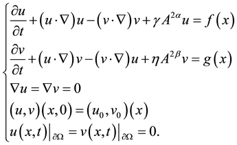
In this paper, we study the following magnetohydrodynamic system:
 (1.1)
(1.1)
here  is bounded set,
  is the bound of
 , where u is the velocity vector field, v is the magnetic
vector field,  are the kinematic viscosity and diffusivity constants respectively.
 . Let
. Let .
.
When , problem (1.1) reduces to the MHD equations. In particular, if
 , problem (1.1) becomes the ideal MHD equations. It is therefore reasonable to call (1.1) a system of generalized MHD equations, or simply GMHD. Moreover, it has similar scaling properties and energy estimate as the Navier-Stokes and MHD equations.
The solvability of the MHD system was investigated in the beginning of 1960s. In particular in [1] -[4] the global existence of weak solutions and local in time well-posedness was proved for various initial boundary value problems. However, similar to the situation with the Navier-Stokes equations, the problem of the global smooth solvability for the MHD equations is still open.
Analogously to the case of the Navier-Stokes system (see [5] -[8] ) we introduce the concept of suitable weak solutions. We prove the existence of the global attractor (see [9] ) and getting the upper bound estimation of the Hausdorff and fractal dimension of attractor for the MHD system.
2. The Priori Estimate of Solution of Problem (1.1)
Lemma 1. Assume  so the smooth solution
  of problem (1.1) satisfies

Proof. We multiply u with both sides of the first equation of problem (1.1) and obtain
 (2.1)
(2.1)
We multiply v with both sides of the second equation of problem (1.1) and obtain
 (2.2)
(2.2)
According to  we obtain
 (2.3)
(2.3)
According to (2.1) + (2.2), so we obtain
![]() (2.4)
(2.4)
According to Poincare and Young inequality, we obtain
![]() (2.5)
(2.5)
![]() (2.6)
(2.6)
![]() (2.7)
(2.7)
From (2.5)-(2.7), we obtain
![]()
![]()
Let![]() , according that we obtain
, according that we obtain
![]()
Using the Gronwall’s inequality, the Lemma 1 is proved. ![]()
Lemma 2. Under the condition of Lemma 1, and ![]()
![]() ,
, ![]() ,
, ![]() , so the solution
, so the solution ![]() of problem (1.1) satisfies
of problem (1.1) satisfies
![]()
Proof. For the problem (1.1) multiply the first equation by ![]() with both sides, for the problem (1.1) multiply the second equation by
with both sides, for the problem (1.1) multiply the second equation by ![]() with both sides and obtain
with both sides and obtain
![]() (2.8)
(2.8)
![]()
According to the Sobolev’s interpolation inequalities,
![]() (2.9)
(2.9)
![]() (2.10)
(2.10)
According to (2.9)-(2.10), we have
![]() (2.11)
(2.11)
Here
![]()
In a similar way, we can obtain
![]() (2.12)
(2.12)
Here
![]()
![]() (2.13)
(2.13)
Here
![]()
![]()
![]() (2.14)
(2.14)
Here
![]()
![]()
According to the Poincare’s inequalities
![]() (2.15)
(2.15)
![]() (2.16)
(2.16)
![]() (2.17)
(2.17)
From (2.12)-(2.17), we have
![]()
Here
![]()
So
![]()
We obtain
![]()
Using the Gronwall’s inequality, the Lemma 2 is proved. ![]()
3. Global Attractor and Dimension Estimation
Theorem 1. Assume that ![]() and
and ![]() so problem (1.1)
so problem (1.1)
exist a unique solution ![]()
Proof. By the method of Galerkin and Lemma 1-Lemma 2,we can easily obtain the existence of solutions. Next, we prove the uniqueness of solutions in detail.
Assume ![]() are two solutions of problem (1.1), let
are two solutions of problem (1.1), let![]() , Here
, Here ![]() so the difference of the two solution satisfies
so the difference of the two solution satisfies
![]() (3.1)
(3.1)
![]() (3.2)
(3.2)
The two above formulae subtract and obtain
![]() (3.3)
(3.3)
For the problem (3.3) multiply the first equation by u with both sides and obtain
![]() (3.4)
(3.4)
For the problem (3.3) multiply the second equation by v with both sides and obtain
![]() (3.5)
(3.5)
According to
![]() (3.6)
(3.6)
According to (3.1) + (3.2), we have
![]() (3.7)
(3.7)
According to Sobolev inequality, when n < 4
![]() (3.8)
(3.8)
![]() (3.9)
(3.9)
According to (3.8)-(3.9),we can get
![]() (3.10)
(3.10)
![]() (3.11)
(3.11)
![]() (3.12)
(3.12)
![]() (3.13)
(3.13)
From (3.10)-(3.13),
![]()
Here ![]()
So, we have
![]()
![]()
Let![]() , so we obtain
, so we obtain
![]()
According to the consistent Gronwall inequality,
![]()
So we can get ![]() the uniqueness is proved.
the uniqueness is proved. ![]()
Theorem 2. [9] Let E be a Banach space, and ![]() are the semigroup operators on E.
are the semigroup operators on E. ![]() here I is a unit operator. Set
here I is a unit operator. Set ![]() satisfy the follow conditions
satisfy the follow conditions
1) ![]() is bounded. Namely
is bounded. Namely![]() ,
, ![]() , it exists a constant
, it exists a constant![]() , so that
, so that ![]() ;
;
2) It exists a bounded absorbing set ![]() namely
namely ![]() it exists a constant t0, so that
it exists a constant t0, so that ![]() ;
;
3) When![]() ,
, ![]() is a completely continuous operator A.
is a completely continuous operator A.
Therefore, the semigroup operators ![]() exist a compact global attractor.
exist a compact global attractor.
Theorem 3. Assume ![]()
![]()
![]() ,
,![]() . Problem (1.1) have global attractor
. Problem (1.1) have global attractor ![]()
Proof.
1) When ![]() From Lemma 1,
From Lemma 1,
![]()
So ![]() in E is uniformly bounded.
in E is uniformly bounded.
2) ![]() has E in a bounded absorbing set
has E in a bounded absorbing set
![]()
From Lemma 2, when ![]() there is
there is
![]()
Since ![]() is tightly embedded, so
is tightly embedded, so ![]() is
is ![]() in the tight absorbing set in E.
in the tight absorbing set in E.
3) So the semigroup operator ![]() is completely continuous.
is completely continuous. ![]()
In order to estimate the Hausdorff and fractal dimension of the global attractor A of problem (1.1), let problem (1.1) linearize and obtain
![]() (3.14)
(3.14)
Assume ![]()
![]() is the solutions of the problem (3.14). We know
is the solutions of the problem (3.14). We know
![]() . It is easy to prove the problem (3.14) has the uniqueness of solutions
. It is easy to prove the problem (3.14) has the uniqueness of solutions
![]() .
.
To prove ![]() in
in ![]() has differential, let
has differential, let ![]() so there has
so there has
![]()
Theorem 4. Assume ![]() and T are constants, so it exists a constant
and T are constants, so it exists a constant ![]() and
and ![]() has
has ![]()
![]()
![]()
![]()
![]() so there is
so there is
![]() (3.15)
(3.15)
Proof. Meet the initial value problem (3.14) of respectively for![]() ,
, ![]() solutions for
solutions for![]() ,
, ![]() , let
, let![]() ,
,![]() . So
. So![]() ,
, ![]() satisfies
satisfies
![]() (3.16)
(3.16)
Here
![]() (3.17)
(3.17)
![]() (3.18)
(3.18)
For the problem (3.16) multiply the first equation by ![]() with both sides and for the problem (3.16) multiply the second equation by
with both sides and for the problem (3.16) multiply the second equation by ![]() with both sides and obtain
with both sides and obtain
![]() (3.19)
(3.19)
Then
![]() (3.20)
(3.20)
Here![]() .
.
For the problem (3.16) multiply the first equation by ![]() with both sides and for the problem (3.16) multiply the second equation by
with both sides and for the problem (3.16) multiply the second equation by ![]() with both sides and obtain
with both sides and obtain
![]() (3.21)
(3.21)
According to the Sobolev’s interpolation inequalities
![]() (3.22)
(3.22)
![]() (3.23)
(3.23)
According to (3.22)-(3.23), we have
![]() (3.24)
(3.24)
In a similar way, we can obtain
![]() (3.25)
(3.25)
![]() (3.26)
(3.26)
![]() (3.27)
(3.27)
![]() (3.28)
(3.28)
![]() (3.29)
(3.29)
![]() (3.30)
(3.30)
![]() (3.31)
(3.31)
So, we can get
![]()
Here![]() , we obtain
, we obtain
![]()
According to the Poincare’s inequalities
![]() (3.32)
(3.32)
Let![]() ,
,
![]()
According to Gronwall’s inequalities, we obtain
![]() (3.33)
(3.33)
Let ![]() be the solutions of the linear Equation (3.14), and satisfies
be the solutions of the linear Equation (3.14), and satisfies![]() , Assume
, Assume
![]() (3.34)
(3.34)
So, we can get
![]() (3.35)
(3.35)
Here
![]() (3.36)
(3.36)
![]() (3.37)
(3.37)
For the problem (3.33) multiply the first equation by w1 with both sides and for the problem (3.33) multiply the second equation by w2 with both sides and obtain
![]() (3.38)
(3.38)
According to (3.8)-(3.9), then
![]() (3.39)
(3.39)
![]() (3.40)
(3.40)
![]() (3.41)
(3.41)
![]() (3.42)
(3.42)
![]() (3.43)
(3.43)
![]() (3.44)
(3.44)
![]() (3.45)
(3.45)
![]() (3.46)
(3.46)
![]() (3.47)
(3.47)
![]() (3.48)
(3.48)
According to, we obtain
![]()
Here ![]()
![]()
We obtain
![]()
So
![]() (3.49)
(3.49)
Let ![]() be the solutions of the linear Equation (3.33) correspond- ing to the initial value
be the solutions of the linear Equation (3.33) correspond- ing to the initial value ![]() so there is
so there is
![]() (3.50)
(3.50)
![]() is linear mapping that is defined in the problem (3.34),
is linear mapping that is defined in the problem (3.34), ![]() represents the outer product, tr represents the trace, QN is the orthogonal projection from
represents the outer product, tr represents the trace, QN is the orthogonal projection from ![]() to the span
to the span ![]()
Theorem 5. Under the assume of Theorem 3, the global attractor A of problem (1.1) has finite Hausdorff and fractal dimension, and
![]()
Here J0 is a minimal positive integer of the following inequality
![]()
Proof. By theorem [8] , we need to estimate the lower bound of ![]() Let
Let ![]() be the orthogonal basis of subspace of
be the orthogonal basis of subspace of ![]()
![]() (3.51)
(3.51)
According to (3.8)-(3.9), we can get
![]() (3.52)
(3.52)
![]() (3.53)
(3.53)
![]() (3.54)
(3.54)
![]() (3.55)
(3.55)
![]() (3.56)
(3.56)
![]() (3.57)
(3.57)
Under the bounded condition, select ![]() is the standard eigenfunction of
is the standard eigenfunction of![]() ,
, ![]() and the corresponding eigenvalues are
and the corresponding eigenvalues are ![]() and
and
![]()
![]()
Let![]() . Therefore, we can get
. Therefore, we can get
![]()
Let![]() .
.
![]()
By ![]() and
and ![]()
![]()
![]()
So, we can obtain
![]()
We have
![]()
Therefore
![]()
![]()
Funding
This work is supported by the National Natural Sciences Foundation of People’s Republic of China under Grant 11161057.
NOTES
*Corresponding author.