Modelling Textural Anisotropy of Magnetic Susceptibility of Banded Iron Formations ()
1. Introduction
Banded iron formation, usually abbreviated to BIF, is the lithological term for a chemical sediment consisting of a “thinly layered or laminated rock in which chert (or its metamorphic equivalent) alternates with layers that are composed mainly of iron minerals; the iron content typically is in the range 20% - 35% and the SiO2 is in the range 40% - 50%” [1]. High-grade iron ores derived from BIFs form the main reserves of cheaply exploitable iron in Africa, Australia, India, South America, and Russia. Magnetite BIFs in the United States, Canada and China are also mined due to the easy concentration of magnetite by magnetic separation.
Anisotropy of magnetic susceptibility (AMS) of single crystal grains is caused by either magnetocrystalline anisotropy or shape anisotropy [2] [3]. The magnitude of AMS of natural rocks depends on both the anisotropy of individual magnetic particles and the degree of their alignment. The preferred orientation of crystallographic axes commonly controls grain shape and determines the AMS for the vast majority of minerals [4]. The AMS of most natural rocks is formed if there is a net statistical alignment of crystallographic axes, which could be acquired in the original diagenesis, or later metamorphism, deformation and other physical and chemical events. In BIFs, however, ferromagnetic grains are concentrated along some bands. In such a case the magnetic interactions among the ferromagnetic grains can generate an overall magnetic behavior completely different from the behavior of both individual grains and the statistical alignment of crystallographic axes of these grains.
AMS of BIFs is often characterized by high anisotropy [5]-[8] and well-developed bedding-parallel magnetic foliation [7]-[9]. This type of anisotropy was called the textural anisotropy [10]. Since most of previous studies were focused on palaeomagneism of BIFs and BIF-derived iron ores, little effort has been made to further understand this special type of AMS for BIFs. In this paper, some AMS results of Hamersley BIFs are presented. A detailed theoretical analysis is made to understand the mechanism of the formation of this special anisotropy for BIFs. The theoretical model is then tested by the experimental data using artificial BIF samples given in [5].
2. AMS of BIFs in the Hamersley Province
The Hamersley Province in the northwest of Western Australia hosts extensive BIFs and high-grade hematite/martite ores. Fresh BIFs in the Hamersley Province commonly contain ~30 wt% magnetite [11] [12], but they are normally covered by an overlying weathered BIF layer that is tens to ~100 m thick [12]. In weathered BIFs, magnetite content varies from <0.5 wt% to <15 wt% and consequently the bulk susceptibility of weathered BIFs is much lower than that of fresh BIFs. Typical structure of BIFs in the Hamersley Province is shown in Figure 1.
The features of AMS of four selected BIF sites are shown in Figure 2. For each site, the average position of the minimum susceptibility axes is very close to the pole position of bedding, normally with a difference less than 10˚. The average degree of anisotropy of these BIF sites varies from 1.16 to 1.69, and the lineation is almost equal to 1.0. This means that the susceptibility along the bedding is almost isotropic. Thus, all these sites show a well-developed magnetic foliation parallel or sub-parallel to bedding, called textural anisotropy [10].
3. Theoretical Analysis of the Formation of Textural Anisotropy for BIFs
For a standard cylindrical BIF sample (Figure 3), assuming it consists of alternating strong magnetic (intrinsic susceptibility ) and non-magnetic layers (N layers in total). The thickness of each layer, however, can differ. If a magnetic field is applied parallel to the layers, the apparent (or measured) susceptibility of the whole sample parallel to the layer
  is given as [5]:
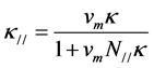 , (1)
, (1)
where  is the volume fraction of magnetic layer material;
  is the demagnetization factor of the sample as a whole in the direction of parallel to the layer.
If a magnetic field is applied normal to the layers, the apparent susceptibility of the whole sample normal to the layer  is given as:
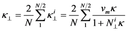 , (2)
, (2)
![]()
Figure 1. Summary of stratification scales within BIFs of the Hamersley Province. White re- presents chert-rich unit and other patterns represent iron-rich unit. Black is for magnetite (modified from [12]).
![]()
Figure 2. AMS of BIFs from Hamersley Province of Western Australia.
![]()
Figure 3. Schematic section of a cylindrical BIF sample.
where  and
and  are the apparent susceptibility and demagnetization factor of the ith magnetic layer in the direction of normal to the layer.
From Equations (1) and (2), the apparent anisotropy  of the sample can be expressed as
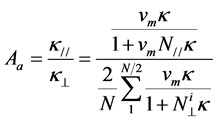 . (3)
. (3)
In case of the equal thickness of each magnetic layer, this apparent anisotropy becomes
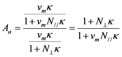 , (4)
, (4)
where 
 is the demagnetization factor of a single magnetic layer normal to the layer. If there is no magnetic interaction between the adjacent magnetic layers,
 ![]() is determined independently by the geometry of a single magnetic layer. For a standard samples,
is determined independently by the geometry of a single magnetic layer. For a standard samples,![]() . Thus Equation (4) is further simplified as
. Thus Equation (4) is further simplified as
![]() . (5)
. (5)
For a thin cylindrical magnetic layer, its demagnetization factor along the cylindrical axis is known as [5]:
![]() (6)
(6)
where p is the length-to-diameter ratio of the cylindrical magnetic layer.
From Equations (5) and (6), theoretical apparent anisotropy of a BIF sample can be determined in the negligence of the inter-layer magnetic action. Figure 4 shows some of these theoretical results, with![]() . It is clear that the apparent anisotropy increases with an increase in intrinsic susceptibility of the magnetic layers (Figure 4(a)), but decreases with an increase in length-to-diameter ratio of the magnetic layer (Figure 4(b)).
. It is clear that the apparent anisotropy increases with an increase in intrinsic susceptibility of the magnetic layers (Figure 4(a)), but decreases with an increase in length-to-diameter ratio of the magnetic layer (Figure 4(b)).
With further increase in the intrinsic susceptibility of the magnetic layers, the apparent anisotropy should differ from these theoretical results. This is because magnetic interactions between the magnetic layers get stronger with increasing intrinsic susceptibility. In such a condition, ![]() in Equation (5) becomes an empirical constant [5], which may be better determined by using contemporary computational methods like neural networks [13] [14] or the combination with statistical means [15], rather than statistics alone.
in Equation (5) becomes an empirical constant [5], which may be better determined by using contemporary computational methods like neural networks [13] [14] or the combination with statistical means [15], rather than statistics alone.
4. Discussion and Conclusion
Jahren [5] gave some experimental results for artificial BIF samples. Some of the results are listed in Table 1. Figure 5 shows the theoretical results of apparent anisotropy using Equations (5) and (6), with a![]() . The corresponding experimental results from Table 1 are plotted and numbered in all the cases.
. The corresponding experimental results from Table 1 are plotted and numbered in all the cases.
Figure 5(a) shows that the two measured points ![]() distribute close to the theoretical curve. This good coincidence continues up to ~1.6 SI. This means that in the case of
distribute close to the theoretical curve. This good coincidence continues up to ~1.6 SI. This means that in the case of ![]() and the adjacent magnetic layers separating by the same ratio, the magnetic interaction between magnetic layers is insignificant when
and the adjacent magnetic layers separating by the same ratio, the magnetic interaction between magnetic layers is insignificant when ![]() SI. Figure 5(b) shows that the three measured points
SI. Figure 5(b) shows that the three measured points ![]() are close to the theoretical curve, but
are close to the theoretical curve, but
![]()
Figure 4. Theoretical curves of apparent anisotropy (Aa) versus: (a) intrinsic susceptibility (κ), and (b) length-to-diameter ratio of the magnetic layer (p). The volume fraction of magnetic layer material (vm) is 1/3.
![]()
Figure 5. Theoretical curves of apparent anisotropy (Aa) versus intrinsic susceptibility (κ) with length-to-diameter ratio of the magnetic layer (p) of 0.1250 (a) and 0.0625 (b). Black dots are corresponding experimental results of measured anisotropy using artificial samples in [5]. The volume fraction of magnetic layer material (vm) is ½.
![]()
Table 1. Experimental results of apparent anisotropy of artificial layered samples [5].
this good coincidence can only continue up to <1.5 SI. Point 5 with ![]() SI deviates obviously from the theoretical curve. This is because when the magnetic layers are thinner and closer to each other (p gets smaller), magnetic interactions between the magnetic layers get stronger with increasing intrinsic susceptibility.
SI deviates obviously from the theoretical curve. This is because when the magnetic layers are thinner and closer to each other (p gets smaller), magnetic interactions between the magnetic layers get stronger with increasing intrinsic susceptibility.
Since the real BIF samples are more complicated than the artificial BIF samples, no direct comparison can be made between the theoretical results and the results of the real BIF samples from this study and other previous studies. However, the good correspondence between the theoretical and the measured results from the artificial BIF samples has demonstrated that the banded texture of BIFs is likely to count for the special type of AMS carried by BIFs, i.e., high anisotropy with a well-developed magnetic foliation parallel or sub-parallel to bedding. Thus this study verifies the term of textural anisotropy for BIFs given in [10].