Statistical Analysis of Subsurface Diffusion of Solar Energy with Implications for Urban Heat Stress ()
1. Introduction
Despite a long period of contentious debate, there is now little dissention among scientists who study global climate change that the change is real and likely dominated by human activity [1] . A recent survey of the peerreviewed scientific literature concluded that the number of papers rejecting the consensus on anthropogenic global warming was a “vanishingly small proportion of the published research” [2] .
Evidence for increasing mean global temperature has come from four major sources: 1) the US NASA Goddard Institute for Space Studies (NASA GISS), 2) the US National Oceanic and Atmospheric Administration (NOAA), 3) the UK Climatic Research Unit (CRU), and most recently 4) the US Berkeley Earth Surface Temperature group (BEST) whose acronym reflects what the group believe to be the largest sampling and smallest uncertainties of the major investigations to date [3] .
Reports in both the scientific literature and popular news media have focused nearly exclusively on global aspects of global warming [4] —i.e. on planet-wide catastrophes such as melting of the Antarctic ice sheet, disruption of the thermohaline circulation in the Atlantic, increased frequency and intensity of extreme storm events, and regional perturbations of ecosystems leading to large-scale extinctions. Although global catastrophes are considered within the realm of future possibility, the most serious consequences of climate change to occur soonest will likely be local, not global, and have direct impact on human health [5] , in particular on mortality associated with exposure to ambient temperature [6] .
According to the US Centers for Disease Control and Prevention, heat waves are the most deadly weatherrelated exposure in the US, and account for more deaths annually than hurricanes, tornadoes, floods, and earthquakes combined [7] . Comparable exigencies have also been reported recently for Europe [8] . In measurements of surface land temperatures for the purpose of estimating the background rate of global temperature rise, researchers have systematically excluded measurements in urban areas to avoid the so-called heat-island effect, i.e. the phenomenon that urban areas are ordinarily hotter than rural areas. The effect reflects such urban conditions as fewer trees to provide shade or capture moisture, more asphalt and cement to absorb heat, tall buildings that block heat radiation into space, and other reasons. Thus, the majority of surface temperature studies disregard the principal locations—cities—where impact of temperature change on human living conditions is likely to be the most profound.
Previous attempts have been made to compare urban and rural temperature trends [9] by examining data from surface stations and making statistical adjustments for differences in measurement conditions. Surface temperature measurements, however, are strongly impacted by the variability of daily weather, which increases the uncertainty of low-amplitude trends.
This paper reports on subterranean temperature measurements made over a 5+ year period as a function of time and depth in a medium-size US city (Hartford, Connecticut: ,
, ) and compares the results with surface temperature measurements made in New York City (NYC:
 ,
, ), which is currently the largest US city by population. The two temperature trends are of comparable magnitude, and both are alarmingly higher than the mean regional temperature, which is close to the rate of global temperature rise.
The stochastic process giving rise to the subterranean temperature series can be understood in its essential details as a one-dimensional (1D) heat diffusion process. Knowledge of the diffusion constant, or diffusivity, which was determined from the data in two independent ways, together with shallow subsurface boundary conditions, permits accurate prediction of the temperature series recorded at greatest depth, thereby substantiating the interpretation of the inferred temperature trend. Power spectral analysis of the time series as a function of depth revealed two different power-law variations, which shed further light on underlying stochastic processes.
2. Experimental Procedure and Observed Time Series
Thermal diffusion of solar energy as a function of time and depth was measured by a series of 6 thermistor sensors positioned in a vertical conduit at depths of 10, 20, 40, 80, 160, and 240 cm (uncertainty ) below the surface with cables leading to an above-ground data logger and master computer. The manufacturer-specified operating range of the thermistors is
  with measurement error below
 . The six temperatures were recorded every hour on the hour starting at noon on 7 June 2007. Data analyzed in this paper cover a period of approximately 5.4 years (i.e. through 2012) and comprise
  observations.
A panoramic sample of the resulting time series collected during the first two and a half years and colorcoded for depth is shown in Figure 1. The red trace, designated , from the probe nearest the surface is most sensitive to weather-induced temperature fluctuations, which is the predominant source of noise. With increasing depth d, the corresponding temperature time series
  show diminishing sensitivity to daily
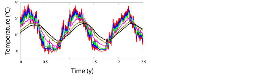
Figure 1. Panoramic plots (truncated to 2.5 y) of hourly temperatures during the period 2007-2012 by sensors at depths (in cm) of 10 (red), 20 (blue), 40 (green), 80 (magenta), 160 (gold), and 240 (black).
weather. The black trace  from the deepest probe, which resembles a smooth sinusoidal function, manifests only seasonal variations in temperature.
The records  and
and  are shown in greater detail in Figure 2. Superposed over the hourly records (red), covering a period of 2000 days, are the 24-hour averaged records
  (black) defined by
 (1)
(1)
for d = 10 and 240 cm, respectively, in which  is the floor function1. At a depth
  daily fluctuations are absent, and there is little difference between
  and
and . Solid black traces close to baseline record the 365-day moving average time series
  defined by
 . (2)
. (2)
It is worth noting that the two kinds of averages are structurally different. In effect, the 24-hour average  replaces each suite of 24 points by 1 point, thereby shortening the input series by a factor of 24. In contrast, the 365-day moving average
  replaces each point by a sum of 365 points, thereby shortening the input series by a length of 365.
3. Abrupt Increase in Rate of Temperature Rise
In combination, transformations (1) and (2) remove nearly all daily and annual variations from the time series. What remains, as shown at larger scale in the plot of  in Figure 3, are weakly varying residuals with long-term trend. The maximum-likelihood (ML) line of regression (heavy dash) yields a rate of temperature increase and standard error of
 . (3)
. (3)
To put this number in perspective, one can compare it to (a) the mean temperature increase for the US Northeast reported by the Union of Concerned Scientists [10]
 (4)
(4)
and (b) the global mean annual temperature rise over the past 30 years reported by the US National Research Council [11]
 . (5)
. (5)
Furthermore, a separate regression analysis (to be published elsewhere [12] ) of above-ground temperature measurements (1960-2012) collected at about 6 km outside the city yielded very close to the same rate as (4). Clearly, the much higher rate of temperature rise (3) is a recent phenomenon.
To ascertain whether  is anomalous among cities, an analysis was made of the time series (1900-2012)
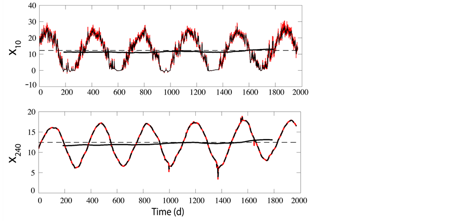
Figure 2. Comparison of hourly (red), 24-hour time-averaged (thin black), 365-day moving average (heavy black), and mean (thin dashed black) temperature records at depths of 10 cm (upper panel) and 240 cm (lower panel).
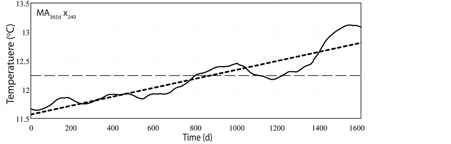
Figure 3. Maximum-likelihood (ML) line of regression (heavy dashed black) to the 365-day moving average temperature series (solid black) recorded at a depth of 240 cm.
of surface temperatures of NYC [13] collected at a station in Central Park, Manhattan. The ML slope and standard error of the line of regression to the time series  for three different spans of time are
 (6)
(6)
The medium-span temperature trend is consistent with the global mean rate (5), and the short-span is consistent with the Hartford rate (3), but larger because NYC has a higher population and population density.
4. Power Spectra and Autocorrelation
Power spectra of the subterranean temperature time series provide detailed information about the stochastic processes by which solar energy propagates through the ground. Of particular interest is the comparison of the spectra of time series  and
and  to confirm that the moving-average series
  is unaffected by daily fluctuations.
To eliminate a static term leading to a zero-frequency spike, time series  were transformed to series
  of zero mean
 . (7)
. (7)
From the Fourier amplitudes of 
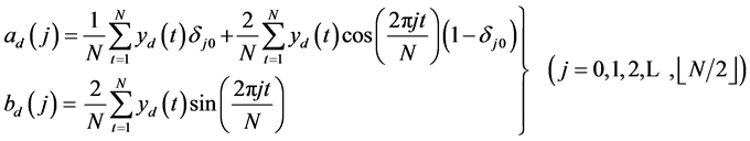 , (8)
, (8)
in which  and
and  is the Kronecker delta function, respectively follow the magnitudesphases, and power spectral amplitudes
 (9)
(9)
 (10)
(10)
 . (11)
For discrete data collected at a sampling rate , the cut-off frequency is
 , beyond which data are aliased, i.e. folded into a lower frequency range. The fundamental
  is the inverse of the duration of the time series. Each frequency
  is labeled by a harmonic number j. The largest harmonic is
  in accordance with Shannon’s sampling theorem [14] .
The harmonic  corresponding to a particular period T (in units of
 ) in a time series of length N is
 , and the time-variation of that harmonic component is then
 . (12)
Figure 4 shows the six waves  of harmonic
  corresponding to annual period
 for a series truncated at
 . These waves reveal the phase shifts and amplitude differences in the large-scale variation of the time series in Figure 1 without accompanying noise.
Of particular interest is the comparison of power spectra obtained from the 10 cm and 240 cm temperature sensors. A double-log plot of , shown in the upper panel of Figure 5, reveals a striking pattern of discrete peaks superposed over a quasi-continuum of harmonics over the range
 . The only other statistically significant peak occurs at
  (not shown), corresponding to the annual period
  2. A double-log plot of
  in the lower panel shows the quasi-continuum of harmonics, but no evidence of discrete peaks. The sequence of discrete peaks, shown separately as a double-log plot in Figure 6, corresponds precisely to the harmonic series3
 of the diurnal period
 . All three double-log plots reveal a power-law dependence
  on frequency
  over the observed range. Regression analysis leads to ML exponents
 (13)
(13)
for the diurnal harmonic spectrum  (Figure 6) and
 (14)
(14)
for the quasi-continuous spectrum  (Figure 5). Exponent (14) is nearly the same for
  upon removal of the diurnal harmonic content.
Further elucidation of the spectral content of  is obtained by examining the power spectra of the 24-hour averaged detrended series
  and the 365-day moving average of the detrended series
  as shown in Figure 7. The oscillatory structure seen in the spectrum of
  does not signify multiple periodicities, but in fact is due entirely to seasonal variability at annual period
 . The sequence of cusps occurs at
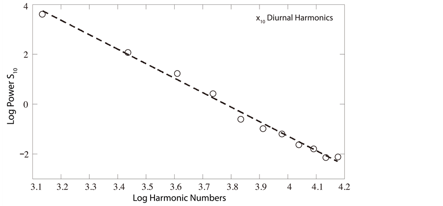
Figure 6. Double-log plot of  (open circles) for the diurnal harmonics
 , superposed by ML line of regression (dashed).
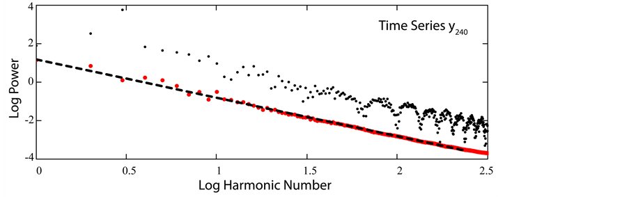
Figure 7. Double-log plots of  (black dots) and
  (red dots) with ML line of regression (dashed black).
frequencies close to where ideally (i.e. in absence of noise) the Fourier transform of a pure sinusoid of period  vanishes, and the log approaches
 . This interpretation is confirmed by the autocorrelation function (red trace) of
  in Figure 8, which is fit exactly by the theoretical autocorrelation function
 (dashed black trace). Upon removal of seasonal variability in the series
 , the sequences of cusps vanishes from the power spectrum in Figure 7 (red dots), which is then fit very closely by a ML line of regression leading to power law exponent
 (15)
(15)
characteristic of 1D Brownian diffusion. The periodicity at  largely vanishes from the autocorrelation in Figure 8 (solid black trace), which then likewise (in accord with the Wiener-Khintchine theorem) manifests a long-range decay characteristic of a Brownian process.
Consider next the statistical distribution of the power spectral amplitudes—or a function of such amplitudes—which is useful in revealing empirically the probability density function (pdf) of a stochastic process. The objective of such an examination is to arrive at a recognizable form of pdf. In Figure 9 are shown histograms of  (upper panel) and
  (lower panel). In appearance the histogram of
  strongly resembles a log hyperbolic density, which is widely found to characterize particle mass and size distributions
in fragmentation processes [15] [16] , as well as stochastic processes involving diffusion of matter, energy or the movement of stock prices [17] . The pdf takes the general form [18]
 (16)
(16)
in which  and
and  are the slopes of the asymptotes of the hyperbolic exponent,
  is a location parameter, and
  is a scaling parameter. The upper panel of Figure 10 shows a histogram of
 , which reveals the hyperbolic form of the exponent in Equation (16) with visually fit asymptotic parameters
 ,
,
 . The histogram of
  in the lower panel of Figure 9 strongly resembles an exponential pdf whose general form is
 . (17)
Correspondingly, a plot of  in the lower panel of Figure 10 reveals the linear form of the exponent in Equation (17) with visually fit parameter
 .
.
Although further investigation of the dynamical origin of these distributions is in progress, for the present purposes it suffices that spectral analysis and autocorrelation have revealed all statistically significant periodicities in the temperature time series.
5. Dynamics of Solar Energy Diffusion
A 1D diffusion model for temperature , based on the heat-flux equation [19]
 , (18)
allows adequate prediction of time series  from the non-stochastic component of
 . The diffusivity
 (19)
(19)
depends on ground thermal conductivity , mass density
 , and specific heat capacity
 . The positive direction of flow (x axis) is into the ground with origin at the surface.
Solving Equation (18) for experimental conditions of this paper leads to
 (20)
(20)
in terms of a theoretically known or empirically determined function  of angular frequency
 . When initial amplitudes
  and phases
  are known for a discrete set of fundamental frequencies
 substitution of
  into (20) leads to the general form
 , (21)
which reduces to
 (22)
(22)
in the case of a detrended time series of single fundamental .
.
Equation (22) permits estimation of the diffusivity D by two independent methods: 1) phase shift between corresponding maxima at times  of two temperature records of known depths
 , (23)
and 2) amplitude attenuation of the peak temperature  recorded at two known depths
 . (24)
Applied to the plots of Figure 4, Equations (23) and (24) led respectively to a mean diffusivity
 . (25)
Given the value  in (25) and the amplitudes and phases
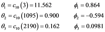 (26)
(26)
from Fourier analysis of the mean-adjusted 3-year temperature record , including contributions at periods
 ,
,  , and
, and  (first diurnal harmonic), one can predict
  from Equation (21), as shown in Figure 11.
The empirical (solid blue) and predicted (dashed black) time series agree very closely in amplitude and phase. The evidence supports the hypothesis that the observed subterranean temperature time series are the result of predominantly one-dimensional solar heat diffusion and that only this solar energy diffusion contributes to the trendline of .
.
6. Conclusions
In contrast to numerous previous studies of global temperature trends by measurements at rural surface stations, this paper reports the measurement and statistical analysis of subterranean temperature within a medium-size city to determine a specifically urban temperature trend. Subterranean measurements at depths of 2 m or more are virtually unaffected by daily temperature fluctuations and are sensitive only to seasonal variations. The mean rate of temperature rise in a medium-size North American city (Hartford CT) between 2007 and 2012, after
transformations eliminating diurnal and seasonal variability, was found to be more than ten times the background rate of global warming. This finding is consistent with surface temperatures recorded in central New York City, the second largest city in North America by population. There is no reason to think that these findings may be atypical for cities in industrialized countries. Given recent occurrences of extreme heat waves in the US and Europe, a precautionary conclusion, substantiated by climate modeling, is that, left unmitigated, the high rate of urban temperature rise relative to global warming will lead to more frequent and intense urban heat stress [20] [21] .
Spectral analysis of the subterranean temperature time series at different depths revealed two distinct power laws suggestive of self-affine fractal behavior over the observed frequency range [22] . The exponent ~2 of the quasi-continuum spectrum is essentially independent of depth and corresponds to fractal Brownian noise (FBN) [23] . In general, FBN with  is more predictable than white noise (WN) for which
 , such as observed in decay of radioactive nuclei [24] . For
 , the future trend follows the past trend, whereas it reverses for
 . Brownian motion with
  lies at the threshold between persistence and anti-persistence because increments are uncorrelated.
The diurnal harmonic spectrum in the shallow subsurface temperature record can be shown [12] to arise from a non-sinusoidal heat flux due to unequal durations of daylight and darkness and the difference in rates of daytime heat absorption and nocturnal cooling. The large power-law exponent ~5.8 characterizes a relatively smooth function with behavior predictable by linear extrapolation. The development of an empirical model that accurately reproduces the diurnal power spectrum for purposes of understanding surface energy fluxes is in progress and will be reported when completed.
Acknowledgements
The author thanks Drs Jon Gourley and Christoph Geiss for several helpful conversations and the staff who maintain the Trinity College Weather Station and Temperature Well. Students who participated at short intervals in the project include Sarthak Khanal, Matthew Cohen, and Robert Tella.
NOTES
1 is the greatest integer less than or equal to n.

2The peak at  theoretically occurs at
 . However, harmonic numbers must be integers.
3The word “harmonic” has two meanings, both of which are used in this paper. In physics, it is a multiple of a fundamental frequency. In mathematics, it is also a series of terms proportional to 
 .
.