Chebyshev Polynomials for Solving a Class of Singular Integral Equations ()
1. Introduction
During the last three decades, the singular integral equation methods with applications to several basic fields of engineering mechanics, like elasticity, plasticity, aerodynamics and fracture mechanics have been studied and improved by several scientists (see [1] -[6] ). Hence, it is interest to solve numerically this type of integral equations (see [7] [8] ). Chebyshev polynomials are of great importance in many areas of mathematics particularly approximation theory (see [9] [10] ).
In this paper we analyze the numerical solution of singular integral equations by using Chebyshev polynomials of first, second, third and fourth kind to obtain systems of linear algebraic equations, these systems are solved numerically. The methodology of the present work expected to be useful for solving singular integral equations of the first kind, involving partly singular and partly regular kernels. The singularity is assumed to be of the Cauchy type. The method is illustrated by considering some examples.
Singular integral equation of first kind, with a Cauchy type singular kernel, over a finite interval can be represented by
 (1.1)
(1.1)
where  and
and  are given real-valued continuous functions belonging to the class Holder of continues functions and
 . In Equation (1.1) the singular kernel is interpreted as Cauchy principle value. Integral equation of form (1.1) and other different forms have many applications (see [1] [2] [6] [11] [12] ). The theory of this equation is well known and it is presented in [13] [14] . An approximate method for solving (1.1) using a polynomial approximation of degree
  has been proposed in [7] .
It is well known that the analytical solutions of the simple singular integral equation
 (1.2)
(1.2)
at  and
and , for the following four cases:
1) The solution is unbounded at both end-points 
2) The solution is bounded at both end-points 
3) The solution is bounded at end  but unbounded at end
 4) The solution is unbounded at end
  but bounded at end
 are given by [15] . In this paper the used approximate method for solving Equation (1.1) stems from recent work [10] wherein an approximate method has been developed to solve the simple Equation (1.2). The approximate method developed below appears to be quite appropriate for solving the most general type Equation (1.1). Some examples are presented to illustrate the method.
2. The Approximate Solution
In this section we present the method of the approximate solution of Equation (1.1) in four cases.
Let the unknown function  in Equation (1.1) be approximated by the polynomial function
 (2.1)
(2.1)
where  are unknown coefficients, to be determined, and in case (I):
 , in case (II):
 , in case (III):
  and in case (VI):
 , where
 ,
,  ,
,  and
and  are The Chebyshev polynomials of the first, second, third and fourth kinds respectively can be defined by the recurrence relations [9] [16] .
 (2.2)
(2.2)
 (2.3)
(2.3)
 (2.4)
(2.4)
 (2.5)
(2.5)
and  are the corresponding weight functions.
Substituting the approximate solution (2.1) for the unknown function into (1.1) yields
 (2.6)
(2.6)
In above Equation (2.6), we next use the following Chebyshev approximation to the kernels  and
and , given by (for fixed
 , cf. [7] )
 (2.7)
(2.7)
with known expressions for  and
and . Then (2.6) gives
 (2.8)
(2.8)
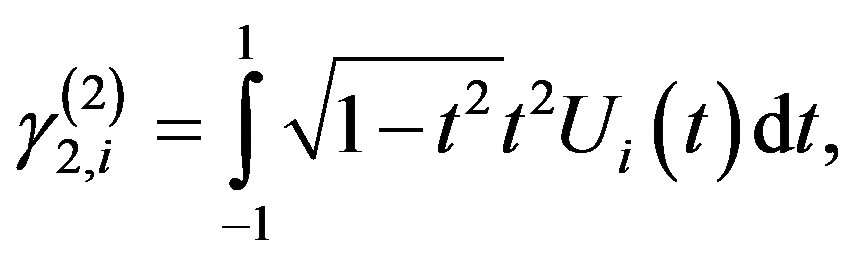
where
 (2.9)
(2.9)
with
 (2.10)
and
 (2.11)
Let , be the zeros of
  and
and , respectively. Substituting the collocation points
  into (2.8) we obtain the following systems of linear equations:
 (2.12)
where
 (2.13)
Solving the system of Equation (2.12) for the unknown coefficients , and substituting the values of
  into (2.1) we obtain the approximate solutions of Equation (1.1).
3. Numerical Examples
In this section, we consider some problems to illustrate the above method. All results were computed using FORTRAN code.
Example 1 Consider the following singular integral equation
 (3.1.1)
where . So, one gets


Hence we find that relation (2.8) produces

Thus (2.9) gives

Firstly, let us consider in detail the case (I),  , for
, for . This results in
 (3.1.2)
 (3.1.3)
By applying the following relations
 (3.1.4)
 (3.1.5)
It is easy to estimate the values  and
and .
.
From (2.2) and (3.1.2)-(3.1.5) we get
 (3.1.6)
By choosing the collocation points , for
, for  we obtain the following system of linear equations:

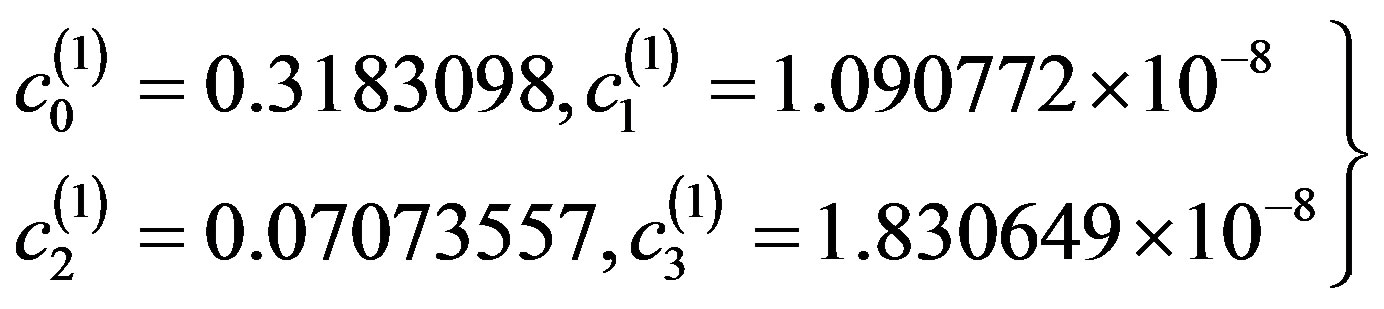
By solving this system for the unknown coefficients  that produces
 (3.1.7)
From (3.1.7) we obtain the approximate solution of Equation (3.1.1) in the form
 (3.1.8)
Which coincides with the exact solution. The error of approximate solution (3.1.8) of Equation (3.1.1) at  is given by Table 1.
Secondly, let us consider in detail the case (II),  , for
, for . This results in
 (3.1.9)
 (3.1.10)
By applying the following relations
 (3.1.11)
 (3.1.12)
It is easy to estimate the values  and
and .
.
From the relations (2.3) and (3.1.9)-(3.1.12) we get
 (3.1.13)
By choosing the collocation points , for
, for  we obtain the following system of linear equations :

By solving this system for the unknown coefficients  that produces
 (3.1.14)
From (3.1.14) we obtain the approximate solution of Equation (3.1.1) in the form
 (3.1.15)
Which coincides with the exact solution. The error of approximate solution (3.1.15) of Equation (3.1.1) at  is given by Table 1.
Thirdly, let us consider in detail the case (III),  , for
, for . This results in
 (3.1.16)
 (3.1.17)
By applying the following relations
 (3.1.18)
 (3.1.19)
It is easy to estimate the values  and
and .
.

Table 1. Illustrates errors of approximate solutions of Equation (3.1.1) in Cases (I)-(IV) at n = 20.
From the relations (2.4) and (3.1.16)-(3.1.19) we get
 (3.1.20)
By choosing the collocation points , for
, for  we obtain the following system of linear equations :

By solving this system for the unknown coefficients  that produces
 (3.1.21)
From (3.1.21) we obtain the approximate solution of Equation (3.1.1) in the form of
 (3.1.22)
Which coincides with the exact solution. The error of approximate solution (3.1.22) of Equation (3.1.1) at  is given by Table 1.
Fourthly, In case (IV),  , for
, for . This results in
 (3.1.23)
 (3.1.24)
By applying the relations
 (3.1.25)
 (3.1.26)
It is easy to estimate the values  and
and .
.
From the relations (2.5) and (3.1.23)-(3.1.26) we get
 (3.1.27)
By choosing the collocation points , for
, for  we obtain the following system of linear equations :

By solving this system for the unknown coefficients  that produces
 (3.1.28)
From (3.1.28) we obtain the approximate solution of Equation (3.1.1) in the form of
 (3.1.29)
which coincides with the exact solution. The error of approximate solution (3.2.29) of Equation (3.2.1) at  is given by Table 1.
Example 2. Consider the following singular integral equation
 (3.2.1)
which corresponds with  and
and . So one gets


Hence we find that relation (2.8) produces

Thus (2.9) gives

Firstly, let us consider in detail the case (I),  , for
, for . This results in
 (3.2.2)
From the relations (3.1.2)-(3.1.5) and (3.2.2) we obtain
 (3.2.3)
By choosing the collocation points , for
, for  we obtain the following system of linear equations :

By solving this system for the unknown coefficients  that produces
 (3.2.4)
From (3.2.4) we obtain the approximate solution of Equation (3.2.1) in the form of
 (3.2.5)
which coincides with the exact solution. The error of approximate solution (3.2.5) of equation (3.2.1) at  is given by Table 2.
Secondly, let us consider in detail the case (II),  , for
, for . This results in
 (3.2.6)
By applying the relations (3.1.9)-(3.1.12) and (3.2.6) we get
 (3.2.7)
By choosing the collocation points , for
, for  we obtain the following
Table 2. Illustrates errors of approximate solutions of Equation (3.2.1) in Case (I), Case (II) and Case (IV) respectively at n = 20.
system of linear equations:

By solving this system for the unknown coefficients  that produces
 (3.2.8)
From (3.2.8) we obtain the approximate solution of Equation (3.2.1) in the form of
 (3.2.9)
which coincides with the exact solution. The error of approximate solution (3.2.9) of Equation (3.2.1) at  is given by Table 2.
Thirdly, In case (IV),  , for
, for . This results in
 (3.2.10)
By applying the relations (3.1.23)-(3.1.26) and (3.2.10) we get
 (3.2.11)
By choosing the collocation points , for
, for  we obtain the following system of linear equations:

By solving this system for the unknown coefficients  that produces
 (3.2.12)
From (3.2.12) we obtain the approximate solution of Equation (3.2.1) in the form of
 (3.2.13)
which coincides with the exact solution. The error of approximate solution (3.2.13) of Equation (3.2.1) at  is given by Table 2.
Similarly, doing the same operations as we did for Case (I), Case (II) and Case (IV), one can solve for Case (III) .
Example 3. Consider the following singular integral equation
 , (3.3.1)
which corresponds with  and
and . So, one gets


Hence the relation (2.8) produces
 (3.3.2)
where (2.9) gives

Firstly, let us consider in detail the case (II),  , for
, for . From (3.1.9)-(3.1.12) and (3.2.6) we get
 (3.3.3)
By solving the system (3.3.2), at the collocation points , for the unknown coefficients
  we obtain
 (3.3.4)
So the approximate solution of Equation (3.3.1) is given by
 , (3.3.5)
which coincides with the exact solution, the error of the approximate solution (3.3.5) of Equation (3.3.1) at  is given by Table 3.
Secondly, in case (III),  , for
, for . This results in
 (3.3.6)
From (3.1.16)-(3.1.19) and (3.3.6) we get
 (3.3.7)
By solving the system (3.3.2), at the collocation points , for the unknown coefficients
  we obtain
 (3.3.8)
Hence, the approximate solution of Equation (3.3.1) is given by
 (3.3.9)
which coincides with the exact solution, the error of the approximate solution (3.3.9) of Equation (3.3.1) at  is given by Table 3.
Table 3. Illustrates errors of approximate solutions of Equation (3.3.1) in Case (II) and Case (III) at n = 20.
Similarly, doing the same operations as we did for Case (II) and Case (III), one can solve for Case (I) and Case (IV).
4. Conclusion
Numerical results (Tables 1-3) show that the errors of approximate solutions of Examples 1-3 in different Cases with small value of n are very small. These show that the methods developed are very accurate and in fact for a linear function give the exact solution.