Application and Generalization of Eigenvalues Perturbation Bounds for Hermitian Block Tridiagonal Matrices ()
Keywords:
Theorem 2.1 [2]. Let  and
and  be n-by-n Hermitian matrices. Let
  and
and  denote the ith smallest eigenvalues of
  and
and , respectively. Then for
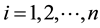 , we have
 (1.1)
(1.1)
where all the eigenvalues of  and
and  are indexed in ascending order.
This is the Weyl’s theorem, which is one of the most classic eigenvalue perturbation theories. When the perturbation matrix  is an arbitrary Hermitian matrix, the bounds obtained by Weyl’s theorem can be very small. However, for Hermitian matrices with special sparse structures such as block tridiagonal Hermitian matrix, the Weyl’s theorem may not be the best choice. For this reason, [1] considered the difference between eigenvalues of the block tridiagonal Hermitian matrices
  and
and , where
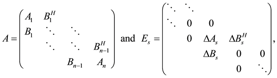 (1.2)
(1.2)
in which  are Hermitian matrices and
  are arbitrary
matrices, the perturbation matrices  and
and  have the same order with the matrices
  and
and , respectively. Let
  and
and  denote the ith smallest eigenvalues of matrices
  and
and , respectively. Let
 denote the set of all the eigenvalues of the Hermitian matrix
 . By defining
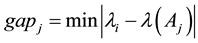 , and assuming that there exists an integer
  such that
 , the
, the
paper [1] obtained the shaper eigenvalue perturbation bounds
 (1.3)
(1.3)
in which
and

The natural questions are that whether the above results can be used to estimate the perturbation bounds for singular values of a block tridiagonal matrix, and how to get the eigenvalues perturbation bounds when two adjacent blocks of the matrix  in the formula (1.2) are perturbed simultaneously. If we apply the results above repeatedly, we can obtain a weaker upper bounds. Inspired by these questions, in this paper, we expect to obtain the perturbation bounds for singular value of a block tridiagonal matrix. Further, we give a new idea to obtain the eigenvalues perturbation bounds by directly using the bounds of eigenvector elements rather than applying the results in [1] repeatedly.
The structure of this paper is organized as follows. In Section 2, we provide preliminaries to outline our basic idea of deriving eigenvalue perturbation bounds via bounding eigenvector components [1]. In Section 3, we present a new approach to estimate the perturbation bounds for the singular values of the block tridiagonal matrix via applying the ideas in paper [1]. In Section 4, we consider the case which the sth block and  block of the matrix
  are perturbed simultaneously and present a new perturbation bound of the
  smallest eigenvalue
 . Further, we discuss the eigenvalue perturbation bounds when the first
  blocks of
  are perturbed simultaneously and provide an algorithm to estimate the bounds. In Section 5, we present a numerical example to show the efficiency of our approach.
Notations. Let  denote the matrix spectrum norm.
2. Preliminaries
For simplicity, the eigenvalues that we mention in this paper are all simple eigenvalues. We need the following conclusion about the partial derivative of simple eigenvalue of  for further discussion, where
 .
.
Lemma 2.1 [1]. Let  and
and  be n-by-n Hermitian matrices. Denote by
  the ith eigenvalue of
 , and define the vector-valued function
  such that
 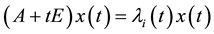 where
where 
for some . If
. If  is simple, then
 (2.1)
(2.1)
Especially, the perturbation matrix  has the special structure. For example, the perturbation matrix
  has the form as the matrix
  whose block elements are zero except for the sth block. Moreover if
  has
has
small components in the positions corresponding to the nonzero elements of , then
  is small. Hence
if we know a bound for the components of  that are in the position corresponding to the nonzero elements
of , then we can obtain a bound for
  via integrating the Equation (2.1) over
 .
.
Yuji Nakatsukasa [1] has derived the eigenvalues perturbation bounds for the case (1.2) with this idea. In the following, we shall describe in detail how this idea can be exploited to derive perturbation bounds of singular values for block tridiagonal matrix, and how this idea is expanded to derive eigenvalue perturbation bounds for our cases.
Note that the Lemma 2.1 holds under the condition that  is a simple eigenvalue of
 . Similarly, we also assume that
  is simple for all
 . For multiple eigenvalues, we can discuss this case by referring to the method of the paper [1,6,7].
3. Singular Value Perturbation bounds
In this section, we use the results in paper [1] to study the perturbation bounds of singular values for the block tridiagonal matrices. For the sake of convenience, we define the sequence of nonzero singular values of a complex  matrix
  by
by
![]()
where ![]() and
and![]() . Similarly, for the perturbation matrix
. Similarly, for the perturbation matrix![]() , we denote the rank of
, we denote the rank of ![]() by
by![]() . Note that the nonzero eigenvalues of
. Note that the nonzero eigenvalues of ![]() and
and ![]() are the same. Generally, the nonzero singular values of
are the same. Generally, the nonzero singular values of ![]() have important applications in many filed, so it's necessary to study singular value perturbation bounds. Just as the discussion of the [1,8] we only consider the simple singular values perturbation bounds.
have important applications in many filed, so it's necessary to study singular value perturbation bounds. Just as the discussion of the [1,8] we only consider the simple singular values perturbation bounds.
3.1. 2 × 2 case
Firstly, for the ![]() case, we have the following results concerning the nonzero singular values perturbation bounds.
case, we have the following results concerning the nonzero singular values perturbation bounds.
Theorem 3.1. Let
![]()
be two complex matrices, ![]() and
and ![]() be the nonzero singular values of
be the nonzero singular values of
![]() and
and![]() , respectively. Define
, respectively. Define![]() ,
, ![]() and
and
![]() . For
. For![]() , if
, if ![]() and the ith singular value
and the ith singular value![]() , then we have
, then we have![]() .
.
Proof. Let
![]() (3.1)
(3.1)
and
![]() (3.2)
(3.2)
By Jordan-Wielandt theorem[2-Theorem I.4.2], we know that the eigenvalues of the matrix ![]() are
are![]() , where
, where![]() . The same statement holds for
. The same statement holds for![]() . Permuting the rows and columns of the matrix
. Permuting the rows and columns of the matrix ![]() appropriately, we can get that the matrix
appropriately, we can get that the matrix ![]() is similar to
is similar to
![]()
and the matrix ![]() is similar to
is similar to
![]()
Let
![]()
Obviously, the matrix ![]() is a
is a ![]() block Hermitian matrix, so is
block Hermitian matrix, so is![]() . Note that the
. Note that the![]() , the eigenvalue set of
, the eigenvalue set of ![]() is
is![]() , and
, and![]() . So it is
. So it is
natural that we can apply the result of [1-Theorem 3.2] to get the conclusion. ![]()
3.2. 3 × 3 case
Secondly, we study the perturbation bounds for singular values of ![]() case. Let
case. Let
![]()
be two complex matrices, where ![]() and
and![]() ,
, ![]() and
and ![]() be the singular values of
be the singular values of ![]() and
and![]() , respectively. Similar to the discussion
, respectively. Similar to the discussion
above, by permuting the rows and columns of ![]() appropriately, we can get that the matrix
appropriately, we can get that the matrix ![]() is similar to
is similar to
![]()
and the matrix ![]() is similar to
is similar to
![]()
Obviously, both ![]() and
and ![]() are block tridiagonal Hermitian matrices. Applying [1-Theorem 4.2], we can get the following theorem.
are block tridiagonal Hermitian matrices. Applying [1-Theorem 4.2], we can get the following theorem.
Theorem 3.2. Let ![]() and
and ![]() be the ith smallest nonzero singular values of
be the ith smallest nonzero singular values of ![]() and
and![]() , respec-
, respec-
tively. Define![]() ,
, ![]() ,
, ![]() and
and ![]() . For
. For![]() , if
, if![]() , then we have
, then we have ![]() .
.
3.3. n × n Case
Further, we gradually consider the general ![]() case and extend above statements to the
case and extend above statements to the ![]() block tridiagonal matrices. Let
block tridiagonal matrices. Let
![]() (3.4)
(3.4)
where ![]() and
and![]() ,
, ![]() and
and ![]() be the nonzero singular values of
be the nonzero singular values of ![]() and
and![]() , respectively. The following conclusion can be demonstrated.
, respectively. The following conclusion can be demonstrated.
Theorem 3.3. Let ![]() and
and ![]() be the ith smallest nonzero singular values of
be the ith smallest nonzero singular values of ![]() and
and![]() , res-
, res-
pectively. Define![]() ,
, ![]() and
and![]() . If there exists a positive integer
. If there exists a positive integer ![]() such that
such that![]() , where
, where![]() , and
, and
![]()
and
![]()
then we have
![]()
In what follows, we give an example to illustrate the singular values perturbation bounds obtained by our results.
Example 3.1. Consider the ![]() matrices
matrices ![]() and
and ![]() represented by
represented by
![]()
where
![]()
Obviously, the last two singular values of ![]() are
are![]() . By computing, we can get that the two singular values of
. By computing, we can get that the two singular values of ![]() are
are
![]()
Therefore, we can get
![]() (3.5)
(3.5)
Through the Theorem 3.1 we know that
![]()
By comparing the differences in the equation (3.5) with the bounds obtained by the Theorem 3.1, we can find that the singular values perturbation bounds obtained by the Theorem 3.1 are sharp and this estimating method is efficient.
4. Eigenvalue Perturbation Bounds
On the basis of conclusions of the paper [1], in this section we study eigenvalue perturbation bounds of block tridiagonal matrix for the cases where two adjacent blocks of ![]() are perturbed and the first
are perturbed and the first ![]() blocks of
blocks of ![]() are perturbed by the perturbation matrix
are perturbed by the perturbation matrix![]() .
.
4.1. Two adjacent blocks of A Being Perturbed
In this subsection, we discuss eigenvalue perturbation bounds when two adjacent blocks of ![]() are perturbed. In other words, we consider the matrices in the following form
are perturbed. In other words, we consider the matrices in the following form
![]() (4.1)
(4.1)
Similar to discussion of the paper [1], we need the following assumption.
Assumption 1. There exists an integer ![]() such that
such that![]() , where
, where ![]()
Roughly, the assumption demands that ![]() is far away from the eigenvalues of
is far away from the eigenvalues of![]() , respectively, and the norms of
, respectively, and the norms of ![]() and
and ![]() are not too large.
are not too large.
Now, on the basis of the Assumption 1, we first discuss upper bounds for the eigenvector components of the matrix![]() .
.
Lemma 4.1. Let ![]() and
and ![]() be Hermitian block-tridiagonal matrices in (4.1),
be Hermitian block-tridiagonal matrices in (4.1), ![]() be the ith smallest
be the ith smallest
eigenvalue of![]() . For
. For![]() , let
, let![]() , where
, where ![]() and
and
![]() satisfying that
satisfying that ![]() and
and ![]() have the same number of rows. Define
have the same number of rows. Define
![]()
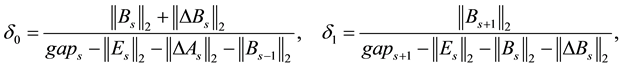
and for![]() ,
,
![]() (4.2)
(4.2)
If ![]() satisfies Assumption 1, then, for all
satisfies Assumption 1, then, for all ![]() we have
we have
![]() (4.3)
(4.3)
Proof. The first block component of ![]() is
is
![]()
Since ![]() for
for![]() , by Weyl’s theorem,
, by Weyl’s theorem,
we have![]() . Therefore, we have
. Therefore, we have
![]()
Further, by applying the Theorem 2.1[2], we know ![]() and
and
![]() . So we can bound
. So we can bound ![]() by
by
![]() (4.4)
(4.4)
where the right inequality follows from Assumption 1. Continuously, the second block component of
![]() is
is
![]()
So,
![]()
Similarly, by Weyl's theorem, we have![]() . Combining this inequality with
. Combining this inequality with
(4.4), we can get
![]()
Hence,![]() .
.
By the same argument, we can prove ![]() for all
for all ![]()
To consider the sth block component of![]() , we have
, we have
![]()
thus,
![]()
By using the results of the Assumption 1 and Theorem 2.1[2], we know that ![]() is invertible
is invertible
and![]() . Since
. Since![]() , we can get
, we can get
![]()
Therefore, for all ![]() we can obtain the following result
we can obtain the following result
![]()
Continuously, considering the s + 1th block of![]() ,
,
![]()
we have
![]()
Similarly, by using the results of the Assumption 1 and Theorem 2.1[2], we know that ![]()
is invertible and![]() . Since
. Since![]() , for all
, for all
![]() , we can get
, we can get
![]()
Hence,
![]()
Similar to the discussion above, we also have
![]()
![]()
By ![]() and
and![]() , we have
, we have
![]()
Consequently, for all![]() ,
,
![]()
Similar to the discussion above, we can prove![]() . In addition,
. In addition,![]() .
.
Based on the discussion above, we conclude that for all![]() ,
,
![]()
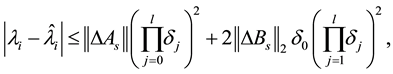
The following Theorem 4.1 is aiming to present perturbation bounds for![]() .
.
Theorem 4.1. Let ![]() and
and ![]() be the
be the ![]() smallest eigenvalues of matrix
smallest eigenvalues of matrix ![]() and
and![]() , respectively, and
, respectively, and ![]() be defined as in (4.2). If
be defined as in (4.2). If ![]() satisfies the Assumption 1, we have
satisfies the Assumption 1, we have
![]()
Proof. Integrating (2.1) over ![]() we get
we get
![]()
Together with (4.3), it follows that
![]()
4.2. The first s blocks of A Being Perturbed
In this subsection, we gradually consider the bounds of eigenvalues of the matrix![]() , whose the first
, whose the first ![]() blocks are perturbed simultaneously. In other words, we consider the perturbation matrix
blocks are perturbed simultaneously. In other words, we consider the perturbation matrix
![]() (4.5)
(4.5)
where ![]() is a positive integer.Let
is a positive integer.Let ![]() denote the ith eigenpair of
denote the ith eigenpair of ![]() satisfying
satisfying
![]() , and the partition of
, and the partition of ![]() satisfies that
satisfies that ![]()
and ![]() have the same number of rows, where
have the same number of rows, where![]() .
.
If ![]() satisfies the Assumption 1, through the similar discussion as above, we can derive a similar conclusion for calculating the eigenvalue perturbation bounds. For simplicity, we don't repeat the proof here. The Algorithm 1 below shows the calculation in detail, where
satisfies the Assumption 1, through the similar discussion as above, we can derive a similar conclusion for calculating the eigenvalue perturbation bounds. For simplicity, we don't repeat the proof here. The Algorithm 1 below shows the calculation in detail, where![]() ,
, ![]() and
and![]() .
.
5. Numerical Example
In this section, we use the following example to illustrate the validity of our method and to show the advantage of the our method over the method proposed in [1].
Example 5.1 [1]. Let ![]() be the
be the ![]() tridiagonal matrix
tridiagonal matrix
![]() (5.1)
(5.1)
Algorithm 1. Eigenvalue perturbation bound algorithm for the first s blocks of ![]() being perturbed.
being perturbed.
where all the elements of ![]() are zero except for the 900th and 901th off diagonal, which are 1
are zero except for the 900th and 901th off diagonal, which are 1![]() . Note that none of the off-diagonals is negligibly small. We focus on
. Note that none of the off-diagonals is negligibly small. We focus on ![]() (the ith smallest eigenvalue of
(the ith smallest eigenvalue of![]() ) for
) for![]() , which are smaller than 10. For such
, which are smaller than 10. For such ![]() we have
we have![]() , and give bounds for
, and give bounds for ![]() with our method. The results are outlined in Table 1.
with our method. The results are outlined in Table 1.
Meanwhile, we use the method in the paper [1] to give the perturbation bounds for![]() . The results are outlined in Table 2.
. The results are outlined in Table 2.
Further, we partition the matrix ![]() as in the (5.1) again so that the block size is one except for the 900th
as in the (5.1) again so that the block size is one except for the 900th
block, which is 2-by-2 matrix![]() . In other words, we set
. In other words, we set![]() ,
, ![]() , and set
, and set![]() ,
, ![]() (i.e., s = 900). Using the method in the paper [1] we have the following
(i.e., s = 900). Using the method in the paper [1] we have the following
perturbation bounds for![]() , which are outlined in Table 3.
, which are outlined in Table 3.
Obviously, comparing the table 1 with the table 2, we can see that our method saves CPU times and improves the perturbation bounds. In addition, comparing the table 1 with the table 3, although our CPU time is close to the CPU time in Table 3, we see that the perturbation bounds are also improved . So we can say that our method is efficient and improved.
6. Conclusion
We have obtained a new efficient method to estimate the perturbation bounds for singular values of block tridiagonal matrix. Further, under the bases of the paper [1], we present a new conclusion for estimating the perturbation bound when the sth block and ![]() block of the matrix
block of the matrix ![]() are perturbed simultaneously and
are perturbed simultaneously and
![]()
Table 1. The eigenvalue perturbation bounds and CUP times.
![]()
Table 2. The eigenvalue perturbation bounds and CUP times.
![]()
Table 3. The eigenvalue perturbation bounds and CUP times.
provide an algorithm for the general case when the first ![]() blocks of
blocks of ![]() are perturbed simultaneously. Number examples are presented to show the effectiveness of our methods.
are perturbed simultaneously. Number examples are presented to show the effectiveness of our methods.
References
NOTES
*The work was supported by the Fundamental Research Funds for the Central Universities (xjj20100114) and the National Natural Science Foundation of China (11171270).
#Corresponding author.