Keywords: Carrying Capacity; Non-Linearity; Multiplicative Fluctuations; White Noise; Fokker-Planck Equation; Periodic Phenomena; Erlang Distribution
1. Introduction
Resources generated through bio-reproduction processes and through bio-chemical processes constitute a rare and unique gift of the nature to the human race. These resources are renewable by the very nature of biological processes. Fishery is a prime example of renewable resources that the human race has been exploiting for its survival and shelter since the time immemorial. Fresh water resources are repeatedly renewed through the nature’s recurrent activities, and in turn they renew our agricultural produces and hydro-electric power generation [1-2]. The problem of management is complicated by the factor that the natural populations have a tendency to fluctuate in response to stochastic perturbations in their physical and/or biological environment [3]. Further, it has been observed that models proposed for fish growth as well as other neoclassical growth models in this direction are described by a relevant first order ordinary differential equation. However, it has been recently observed that most of the fishery processes are non-linear and stochastic in nature; and during the foregoing decade a great deal of research work has been pursued to elucidate the role of nonlinearity and stochasticity in the evolution of the processes. Most of the work incorporating nonlinearities and stochasticity is either empirical or of qualitative in description. We have been motivated to make a theoretical attempt to study stochastic logistic models of fish growth.
2. Deterministic Model
As a matter of fact, after the success achieved by Pearl [4] in fitting logistic formula
 (1)
(1)
or the corresponding differential equation
 (2)
(2)
where  is the intrinsic growth rate per unit, K is the carrying capacity of the system and are constants including
 . The logistic law has been applied in biology both to experimental populations and to the growth of individuals. Feller [5], has demonstrated in quite clear cut terms that even a good agreement of the logistic law with actual observations does not in itself imply the correctness of the biological assumptions underlying the mathematical deduction of the logistic law. Further, it has been observed that the same logistic law is not applicable to the different fish population [6].
In the first stage of the extensions, we shall remain confined to the deterministic versions. A close scrutiny of Equation (2) shows that it may be immediately modified in the following ways: Faris Laham et al. [7] have observed periodic phenomena occurring in the realm of Tilapia fish. Let us also recall that the basic features of a logistic growth rate are deeply influenced by the carrying capacity of the system. Therefore, it is quite logical and natural to consider the carrying capacity  changes periodically with time and consequently, we set
 (3)
(3)
If  is the period of oscillations in the carrying capacity then the frequency
 , and the angular frequency
  are connected through
 (4)
(4)
The units of  are to be taken as radians per unit time. We shall carry out the analysis of this case in the following section.
Further, it has been observed that some fish species are grow rapidly and some are very slowly. Thus, in the former case, the growth curve lies to the left and above of the logistic curve, while in the later case, the growth curve lies far to the right and below the logistic curve. Bearing these points in mind, we propose the second extension of Equation (2) in the form
 (5)
(5)
where  denotes the fish population size at time
 , with
 . And
. And , are constants along with
 .
.
3. Deterministic Analysis of the Extension Models
Case-I: Substituting Equation (3) into Equation (2), we obtain
 (6)
(6)
Setting,  and
and  in Equation (6), we have
 (7)
(7)
Further, assuming that , Equation (7) can be approximated to
 (8)
(8)
In order to convert the non-linear Equation (8) into linear equation we have to use the transformation
 , (9)
, (9)

or
 (10)
(10)
with initial condition
 (11)
(11)
The integration of the non-homogeneous linear Equation (10) and using the initial condition Equation (11), we obtain
 (12)
(12)
where

The asymptotic behavior of Equation (12) will be governed by
 (13)
(13)
Case-II: Regarding the second extension given by Equation (5), we have already pointed out the expected qualitative changes. First of all we observe that Equation (5) is also a non-linear equation of Bernoulli type, hence it can be reduced to a linear equation by setting
 (14)
(14)
Rearrangement of Equation (5) leads to

or
 (15)
(15)
Combining Equations (14) and (15), we find
 (16)
(16)
with initial condition, 
The direct integration of Equation (16) gives

or
 (17)
(17)
For large , Equation (17) becomes
 (18)
(18)
and
 (19)
(19)
As in the Case-I, we observe here that, in long-run the fishery process effectively forget its initial stage, however, the choice of  remarkably control the growth.
4. Stochastic Formulation of the Extension Model (Case-I)
Stochastic Formulation of the Extension Model (Case-I): Several stochastic versions of logistic model have been discussed in literature on population processes and in ecology [8-11], and only the steady-state studies have been made. In our problem, we shall first obtain a time dependent solution of stochastic version of the logistic version of the logistic model for fish growth with multiplicative fluctuations. The stochastic differential equation corresponding to Equation (2)
 (20)
(20)
with initial condition 
where  is a positive constant, solely depending on the prevailing fluctuations in the reservoir and can be evaluated from the data on the process.
  is standard White noise with zero mean and unit intensity and is independent of
 . For the sake of clarity and brevity, we shall rewrite Equation (20) as
 (21)
(21)
where .
.
On setting , the non-linear Equation (21) reduces to the linear equation
 (22)
(22)
with initial condition 
Using the concept of White noise, we obtain the drift and diffusion coefficients  and
and  of the process
 .
.
 (23)
(23)
The corresponding probability density function  with an initial value
  satisfies the Fokker-Planck Equation (FPE)
 (24)
(24)
Further, if we transform  to a new set of variables
  such that
  and
and  then
then  transforms to a new probability density function
 . Now ignoring the Jacobian
 , which will appear throughout, we find
 (25a)
(25a)
or
 (25b)
(25b)
or
 (25c)
(25c)
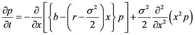
Therefore, on substituting Equation (25a) to Equation (25c) into Equation (24), we obtain
 (26)
(26)
where

For the sake of compactness, we shall rewrite Equation (26) as
 (27)
(27)
where


Therefore, Equation (27) becomes
 (28)
(28)
In this setting, following Wang and Uhlenbeck [12], the function  can be interpreted as variance of
 , and the Equation (28) can be considered as continuity equation for the probability density, and
 (29)
(29)
as the probability flux.
Further, following Feller [13], we consider the boundaries  and
and  as reflecting barriers, and we thus have
 (30)
(30)
Equation (28) with boundary conditions, Equation (30), can be solved either by using the method of separation of variables or by applying the Laplace transformation technique. In the former case the partial differential Equation (28) is transformed into two ordinary differential equations of order one and two, whereas in the later case we obtain a single non-homogeneous ordinary differential equation of order two. However, the second approach becomes tedious and involved for two reasons. Firstly, to solve the Laplace transform of Equation (28), we have to construct suitable Green’s functions; and secondly the Laplace inversion of the solution so obtained in itself is a formidable task. In our study, therefore, we shall adhere to the former method.
5. Solution of the Problem
We split up our probability density function  in such a way that the partial differential equation Equation (27) transforms into two ordinary differential equations. Keeping in view that the limiting distribution
  should result into the steady-state distribution,
  , we set
 (31)
(31)
where  depends on
  and
and  and
and  depend on
  only. Substituting Equation (31) into Equation (27), we have
 (32)
(32)
As we have considered  to be the steady-state distribution, so we may write
 (33)
(33)
and therefore Equation (32) reduces to

or
 (34)
(34)
In Equation (34), the left hand side is a function of  alone, whereas the right hand side depends only on
 , so the Equation (34) is a sort of paradox in the sense that, a function of
  is equated to a function of
 , but
, but  and
and  are independent variables. This independence means that the behavior of
  as an independent variable is not determined by
 . The paradox is to be resolved by setting each side equal to
 , a constant of separation. With this setting Equation (34) leads to
 (35)
(35)
and
 (36)
(36)
Now we have two ordinary differential equations Equation (35) and Equation (36) to replace Equation (27). Further, we observe that Equation (27) represents an eigenvalue problem. The boundary conditions Equation (30) imply

or
 (37)
(37)
Using Equation (33) in Equation (37), we obtain the required boundary conditions
 (38)
(38)
6. Determination of First Order pdf F(y)
Since , the integration of Equation (33) yields
 (39)
(39)
where  is a constant of integration. Using the normalization condition, we obtain

Substituting  gives
gives

Whence

and

We can easily show that, treating  as a continuous variable, its steady-state probability density function
  will be given by
 (40)
(40)
With an appropriate identification of parameters, Equation (40) turns out to be an Erlang distribution and, thus in the steady-state the mean and variance can be directly evaluated. Thus on setting  and
and , Equation (40) becomes
 (41)
(41)
Therefore,

and

7. Conclusion
In this paper, first we have investigated the logistic growth rate when it is influenced by the carrying capacity of the system and have analyzed the modified logistic model for fish growth. It is to be highlighted that the different stochastic versions of the logistic model and its extensions can be extended further in several directions. One may examine the threshold effect through logistic model and one can also examine the effect of stochasticity through the parameters  and
and  of the logistic model. In the long-run, the fishery has effectively forgotten its initial perturbation and the persistent behavior is completely described by the particular integral, Equation (13). Further, if the angular frequency of the periodic changes is low compared to the reciprocal of the natural time scale then the amplitude of the size variations is almost equal to the amplitude of the carrying capacity of the system. Beside these, a non-linear equation of Bernoulli type has been transformed to a linear equation so that the overall gross behavior of the simple model be adequate to provide some insight into. Splitting of probability density function provides the partial differential equation into two ordinary differential equations.
[2] K. E. F. Watt, “Ecology and Resource Management,” McGraw-Hill, New York, 1968.
[3] R. G. Coyle, “Management System Dynamics,” Chapter-II, Wiley, New York, 1977.
[4] M. A. Shah and U. Sharma, “Optimal Harvesting Policies for a Generalized Gordon-Schaefer Model in Randomly Varying Environment,” Applied Stochastic Models in Business and Industry, John Wiley & Sons, Ltd., 2002.
[5] R. Pearl, “The Biology of Population Growth,” Knopf, New York, 1930.
[6] W. Feller, “On Logistic Law of Growth and Its Empirical Verification in Biology,” Acta Biotheoretica, Vol. 5, No. 2, 1940, pp. 51-66. http://dx.doi.org/10.1007/BF01602862
[7] J. R. Beddington and R. M. May, “Harvesting Natural Populations in a Randomly Fluctuating Environment,” Science, Vol. 197, No. 4302, 1977, pp. 463-465. http://dx.doi.org/10.1126/science.197.4302.463
[8] M. F. Laham, I. S. Krishnarajah and J. M. Shariff, “Fish Harvesting Management Strategies Using Logistic Growth Model,” Sains Malaysiana, Vol. 41, No. 2, 2012, pp. 171-177.
[9] D. A. Dawson, “Qualitative Behavior of Geostochastic Systems,” Stochastic Processes and Their Applications, Vol. 10, No. 1, 1980, pp. 1-31. http://dx.doi.org/10.1016/0304-4149(80)90002-2
[10] N. Keiding, “Extinction and Exponential Growth in Random Environments,” Theoretical Population Biology, Vol. 8, No. 1, 1975, pp. 49-63. http://dx.doi.org/10.1016/0040-5809(75)90038-6
[11] D. Ludwig, “A Singular Perturbation Problem in the Theory of Population Extinction,” SIAM-AMS Proceedings, Vol. 10, 1976.
[12] M. Turelli, “A Re-Examination of Stability in Randomly Varying versus Deterministic Environments with Comments on the Stochastic Theory of Limiting Similarity,” Theoretical Population Biology, Vol. 13, No. 2, 1978, pp. 244-267. http://dx.doi.org/10.1016/0040-5809(78)90045-X
[13] M. C. Wang and G. E. Uhlenbeck, “On the Theory of the Brownian Motion-II,” Reviews of Modern Physics, Vol. 17, No. 2-3, 1945, pp. 323-342. http://dx.doi.org/10.1103/RevModPhys.17.323
[14] W. Feller, “Diffusion processes in one dimension,” Transactions of the American Mathematical Society, Vol. 77, 1954, pp. 1-31. http://dx.doi.org/10.1090/S0002-9947-1954-0063607-6