A Model Illustrating Consumer Inconstancy: Demand and Supply Sides ()
1. Introduction
John M. Clark, American economist, 1884-1963, in his famous Studies in the Economics of Overhead Costs (1923) writes on the subject of irregularity in economic activity (p. 149):
“Every economic activity has some irregularities, some ups and downs; and these have a way of recurring regularity, or with sufficient approach to regularity so that one may discern an underlying cycle or rhythm. These patterns, cycles, or quasi-cycles are a fascinating as well as an important subject of study. What are their causes? How are they met? Do they mean waste or efficiency? So far as they represent inefficiency for the producers, what means can be adopted to improve the situation, or is no improvement possible or desirable? Do consumers demand irregularity, consciously or unconsciously? Do those who demand it pay what it cost? Would they demand it if they had to pay what it costs? Does anyone know what it costs?”
In this paper, we present a model that can be a theoretical beginning to answer some of Clark’s questions on irregularity in economic activity.
2. John M. Clark: Does Anyone Know What Demand Irregularity Costs?
2.1. Definition of the Model and Its Terms
We assume a single homogeneous perishable or semiperishable product,  , much like cement [1]. We assume competitive manufacturing SRMC pricing behavior, and ease of entry of new producers. We assume two states of demand,
  and
and , off-peak and peak, each with a likelihood, where the likelihoods add to one. Producers can choose between two technologies to manufacture
 , technology
 or technology
 . Production plants have durable and specific assets, and linear short-run total cost curves with absolute capacity limits. Technology
 and technology
 differ in per unit variable operating cost
 , per unit capacity costs
  (fixed costs per period divided by maximum production rate per period) and capacity per plant
  (maximum production rate). We envision investors and managers walking into a plant manufacturing store that has two shelves: technology
 (output rigid—the manufacturing of all components, capital intensive or new technology) and technology
 (output flexible—the buying of subcomponents, labor intensive or old technology). On each shelf is a model plant,
  , that costs, say, $1,000,000 to build (see Figures 1 and 2). Investors or entrepreneurs can order any multiple or fraction of the model plant of each shelf. No economies of scale exist for each technology. Thus the long-run marginal cost (LRMC) and long-run average cost (LRAC) for all plants in the plant manufacturing store are horizontal.
2.2. Key Assumptions
The key assumptions of the model are:
A1: ,
,  , and
, and  as in Figure 2. The curves in Figure 2 must cross or else the lower one will dominate.
A2: Demand fluctuates with frequencies,  in off-peak and
  in peak and
 .
.
A3: We assume SRMC (short-run marginal-cost) pricing behavior. With linear TC functions and SRMC pricing, producers will operate their plants at either 0% or 100%.
A4: We assume market prices in off-peak times :
:  and market prices in peak times
 :
: . Thus technology
 operates at capacity at all times, while technology
 shutsdown in
  and operates at capacity in
 . In the off-peak period,
  is produced where
  while in the peak period,
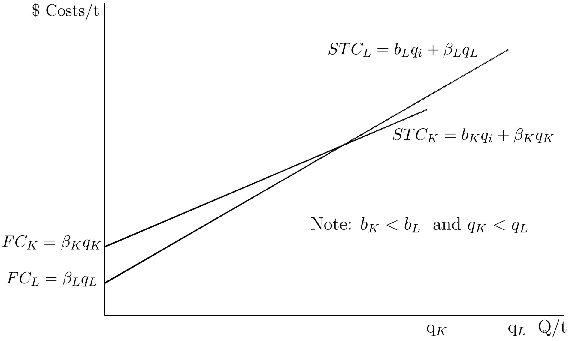
Figure 1. SR total cost curves of 2 plants.

Figure 2. Plant added cost of providing for irregular demand: ABCD.
 is produced where
 .
.
A5: Long-run equilibrium requires zero expected profits for both technologies.
2.3. Objective of Proposition I
We prove in the following proposition the conditions of indifference for investors to choose between technology and technology
 in LR equilibrium.
2.4. Proposition I
Proposition I Under assumptions A1 through A5 with both technologies used in long-run equilibrium, then it must be true:
 (1)
(1)
If  (that is, the left-side inequality is violated) then only technology
 will be used. If
  (that is, the right-side inequality is violated) then only technology
 will be used.
Proof: Applying the zero profit condition to technology :
:
 . (2)
. (2)
This gives us:
 . (3)
. (3)
Applying the zero profit condition to technology :
:
 . (4)
. (4)
This gives us:
 . (5)
. (5)
Equations (3) and (5) can be combined:
 . (6)
. (6)
For plants to shut-down in the off period requires
 , our assumption A4. If
  then, strictly speaking, plants
 are indifferent to producing and some may be producing. Using Equation (6), this requires:
 . (7)
. (7)
Since , We can write:
 (8)
(8)
which is the asserted left-side inequality condition:
 . (9)
. (9)
By assumption A4,  , plants
 to earn a positive contribution margin or all plants, even plants
 , would choose to shut-down in
 . Further,
  because if
 , then positive expected profits to the owners of plants
 would emerge. Thus
 (10)
(10)
yields the right-side inequality condition assertion.
2.5. Left-Side and Right-Side Inequality Conditions
The left-side condition in (1) is that . If one more unit is needed in both peak and off-peak times, the total cost over the cycle of a 1 unit capacity plant producing 1 unit over the cycle is
  since
since . A price of
  will exactly cover costs of one extra unit operating in both periods. We suggest calling this condition that technology
 be more static efficient, in the sense of Clark’s use of the term static in that there are no business cycles [2]1.
The right-side condition in (1) is that
 . Assume we need one more expected unit over the cycle only to meet peak demand. A price of
  will exactly cover costs of one extra expected unit over the cycle operating only in high-demand.
The right-hand condition is that where production is used only in high-demand times, technology is superior. The right-hand condition requires that SAC
 be flatter shaped than SAC
 . We define output flexibility as the relative flatness of the SAC curve. We suggest calling this condition that technology
 be more output-flexible efficient. We cited elsewhere Clark’s writing on the importance of retaining old plants and equipment during economic downturns to have their capacity available for economic peak times [3].
2.6. The Added Cost of Providing for Irregular Demand
If demand were static with no irregularities, then firms would choose only technology and
and . Demand is irregular in the model, fluctuating between
  and
and . The added cost of providing for irregular demand in the model is borne entirely by technology
 where
where .
.  .
.
Thus, a measure of added cost of providing for irregular demand in the model would be the expected quantity produced in peak demand  the difference in SRAC between the two technologies, or:
  . See Figure 2 which shows the added cost of providing for irregular demand for a single plant
 (rectangle ABCD).
Rectangle ABCD shows, in the model of the paper [3], the added cost to have output-flexible technology, technology , available only to provide for the peak (irregular or inconstant) demand. The investors in plants of technology
 , in the model, get zero expected economic profits over the cycle and so the situation is stable equilibrium. The cost to society in providing for this inconstant demand surge that occurs with
  frequency or likelihood is rectangle ABCD in Figure 2. Consumers are paying, unconsciously, rectangle ABCD,
3. John M. Clark: Do Consumers Demand Irregularity, Consciously or Unconsciously?
3.1. Definition of the Model and Its Terms and Assumptions
There are two groups in our hypothetical society: producers (suppliers) and consumers (households). The households buy standardized semi-perishable food baskets to feed their families. The food baskets have meat, fish, cheese, vegetables, fruits and drinks. Households have no refrigerators and no freezers. They are unable to store food baskets except on Friday for the Sabbath. They are like the Israelites who for forty years in the desert could not save the omer of manna per person from day to day except on Fridays when they could save the extra manna given on Friday for the Sabbath2. Households buy their food baskets in a free market and pay a single market price per food basket for the day. The exception is Friday, when there is the Friday supply price and the Sabbath-day supply price.
Households have a fixed budget for food expenditures. They are price sensitive in purchasing food, in the sense that households will purchase more food at a lower market price and less food at a higher market price.
We assume here that suppliers can handle fluctuations in quantities demanded with infinite ease. We might imagine that suppliers can make long-term contracts for the food at the same cost prices regardless of whether there are wide or narrow differences between weekday and Saturday quantities.
In this model consumers pay a daily market price and obtain daily quantities of food baskets. Consumers pay market price times quantities purchased,  (total revenue to suppliers equals market price times quantities).
The demand curve shows the maximum quantities consumers would be willing to purchase at various prices. The area under the demand curve up to the point of quantities of market purchases shows the value to the consumer.
Figure 3 shows a geometric demonstration with
varying pricing (alternative A) versus fixed pricing (alternative B) with fluctuating D functions, weekdays and Sabbath day each with its associated . Let
. Let  be consumer demand for baskets of food (such as meat, fish, bread, cheeses, fruits, vegetables, and drinks) during weekdays, Sunday through Friday. The assumption is that the demand curve is downward sloping, meaning that consumers would be willing to buy more daily if prices were lower, all else being the same.
Using hypothetical numbers to make the economic concepts clearer, point K could be that, at a market price of $36 per basket of food consumers are willing to buy 35 baskets of food per day. Point H might be that at a market price of $33 per basket of food consumers are willing to buy 37 baskets of food per day.
Let D2 be consumer demand for daily baskets of food on the Sabbath. Assume that Sabbath-day food is actually bought on Friday to be eaten on Saturday. Using hypothetical numbers to illustrate, point D could be that, at a market price of $51.9 per basket of food consumers are willing to buy 42 baskets of food per day. Point J could be that, at a market price of $36 per basket of food consumers are willing to buy 54 baskets of food per day.
The demand curve , weekday demand, occurs with frequency,
  , 6/7. The demand curve
 , Sabbath demand, occurs with frequency,
  , 1/7.
We define consumer surplus as the area under the demand curve and above the price line. We define expected values, E, as the sum of each outcome times its expected value. Using the illustrated numbers for points H and D, the market equilibrium points for pricing rule A, varying prices, we can calculate , expected total revenue, and E(Q), expected quantities, as follows:

 .
.
Using the illustrated numbers for points K and J, the market equilibrium points for pricing rule B, fixed prices, we can calculate , expected total revenue, and
 , expected quantities, as follows:

 .
.
3.2. Objective of Proposition II
We prove in the following proposition that consumer surplus is necessarily larger in an arrangement where consumers get more food for the Sabbath at the cost of less food for the weekdays whereby consumers pay the same amount and get the same quantity of food over the week, We show graphically this increase in consumer surplus. This becomes a maximum willingness for consumers to pay suppliers for that arrangement. This is the beginning of creating a demand curve for irregularity.
We assume that suppliers are willing to sell daily according to two alternative pricing schemes: a fixed price,  , at all times, versus
  for weekdays and
  for the Sabbath. We have two basic assumptions in the model: according to both pricing schemes total payments over the week are the same and total food purchases are the same.
We prove that consumers would prefer the scheme whereby they would have extra or more costly food on the Sabbath. In this way they could enjoy the Sabbath more since they would be spending the day with their families and not at work—knowing that they would have less food on the remaining six days. The gain in consumer surplus on the Sabbath,  th of the week, with the extra food when demand for food is high, will outweigh the loss in consumer surplus during the rest of the week,
  th of the week, when there would be less food when demand for food is lower. This is the prescription in Jewish law—to accentuate, as much as possible, the difference between the Sabbath day and the other days of the week, citing Isaiah 58.13: “... call the Sabbath a delight, the holy day of the Lord honored...”
3.3. Proposition II
Proposition II A comparison of alternative pricing schemes, A: varying prices, versus B: fixed prices, under conditions of shifting downward-sloping demand curves shows  and rises as demand elasticity rises assuming
 (11)
(11)
and
 . (12)

Proof: By definition of :
:
 (13)
(13)
and
 . (14)
By definition of :
:
 (15)
(15)
and
 . (16)
By definition of :
:
 (17)
(17)
and
 . (18)
By assumption (11). We can state:
 . (19)
By assumption (12). We can state:
 . (20)
Combining assumptions (11) and (12):
 . (21)
Rearranging:
 . (22)
Using the letters of the Figure 3:
 . (23)
We can state:
 (24)
(24)
Rearranging:
 (25)
(25)
We can state:
 (26)
(26)
Using the results of Equation (23), We can state:
 . (27)
Thus,  must be greater than zero, providing that price elasticities of the demand curves are not zero. At zero price elasticity
  and
and  and therefore areas
  and
and  each equals zero.
  rises as price elasticity rises, since the areas of
  increase with more elastic demand curves.
3.4. Maximum Willingness to Pay for Increased Irregularity
 represents the gain in consumer surplus with fixed pricing over varying pricing that gives the same expected TR to suppliers and same expected Q to consumers. Theoretically
  is a maximum willingness to pay for an arrangement of an increase in irregularity. This is a beginning of constructing a demand schedule for irregularity. The increase in irregularity is going from
  to
to . We could test maximum willingness to pay to increase irregularity further or for a lesser degree of increase irregularity. We could explore the effects on CS with alternative pricing schemes that expected payments rise or expected Q falls.
4. John M. Clark: Man vs. Machine
Clark (1923) points out that people contrast with machines because people want variety and business rhythms of various kinds, while machines, viewed as “a new species of creature” want uniformity and continuous operation. Some business rhythms are predictable such as day/ night and summer/winter. Other business rhythms are unpredictable—the business cycle of recession/prosperity.
Clark, as well as many other economists, argues for methods to make Man accommodate Machine, that is, to reduce cyclicality. How? By pricing policies such as peak-load pricing to induce people to defer purchases from high-demand to low-demand periods. Clark advocates price cuts during slow periods and select reductions to customers when these do not compete with regular sales as ways of getting higher average operating rates and thus economies of full utilization.
5. Conclusions
We provide theoretical models for Clark’s questions: Does anyone know what demand irregularity costs? Do consumers need demand irregularity, consciously or unconsciously?
Our novelty is that, under strict assumptions, consumers prefer business rhythms accentuated, more irregular or inconstant. We argue that output flexibility in technology choice is a way to accommodate consumer demand for inconstancy.
Our research supports the wisdom of John M. Clark [4] who said that consumers have a huge willingness to pay for accentuated fluctuations (triangles KGH + DEJ in Figure 3) with the cost to provide for accentuated and small fluctuations (rectangle ABCD in Figure 2).
NOTES
2Mark that the Lord has given you the Sabbath; therefore He gives you two days’ food on the sixth day. Let everyone remain where he is: let no one leave his place on the seventh day” (Exodus 16: 29).