1. Introduction
In the last two decades an increasing interest has been devoted to studying the impact of endogenous discounting in economic growth models. A bulk of literature postulates that, in sharp contrast with standard neoclassical assumptions, the subjective rate of time preference is not constant, but may depend on some aggregate economic variables, such as individual consumption. The internalization of these external social factors is rich of powerful consequences from the economic point of view, for it leads to a qualitative change in the steady state and its transitional dynamics, so that the perfect foresight equilibrium may not be unique, and thus both local and global indeterminacy can eventually emerge [1,2].
This issue is particularly meaningful in the field of environmental economics, where the economic implications behind global indeterminacy can be interpreted as the way two identically endowed economies (with the same initial stock of both physical and natural capital) may start at some point to follow completely different equilibrium paths towards the long-run steady state. In detail, the rise of multiple equilibria in presence of environmental degradation could be the major cause for a vicious povertyenvironment trap situation, where policies (i.e., technological innovations, resource taxation) aimed at alleviating the overexploitation and exhaustion of the environment which might not be able to avoid a still unsustainable use of natural resources [3-10]. The main implication for any policy decision is that if indeterminacy occurs, public intervention becomes not sufficient to drive the economy towards a good (i.e., less polluting/resource preserving) long-run equilibrium. The agents’ decisions, despite the initial conditions or other economic fundamentals, will locate the economy in a particular optimal converging path that could not coincide with the one corresponding to the lowest extraction levels of natural resources [11,12].
A large strand of analyses demonstrate how a continuum of equilibrium trajectories, existing in the neighborhood of the steady state, can emerge whenever some parametric conditions are verified. This phenomenon is commonly known as local indeterminacy [13-19]. However, only very few attempts have been made to analyze the conditions under which these indeterminacy problems arise outside the small neighborhood of the steady state, which we refer to as global indeterminacy [20]. The latter seems an innovative field to work on, even though it is usually related to very complicated nonlinear functions which increase the mathematical difficulties in handling these models.
This paper explores the implications of endogenous discounting in the framework of a simple optimal growth model with the use of natural resources. Consumption is made at the expenses of environmental quality, the assumption of a constant discount rate of time preference, though it makes the analysis more tractable, can be against the notion of sustainability. To this end, we follow the extant literature on the field, by assuming the dependence of the individual discount rate on the average consumption [21-23]. The novelty of this paper relies on a deep investigation of the global behavior of the economy studied in [24], where indeterminacy may occur for a less stringent set of parametric restrictions. To tackle this problem, we use the principles of bifurcation theory to gain hints on the global properties of the equilibrium, and to investigate the whole set of conditions which lead to the emergence of a quasi-periodic dynamics along an invariant torus. This allows us to better understand the determinants for the emergence of endogenous fluctuations, and the existence of irregular patterns due to a sensitive dependence of our economy on the initial conditions.
The paper develops as follows. The second section introduces the dynamic system associated with [24]. In the third section, we prove the main proposition relating to the global properties of the equilibrium, and show the parametric onset for the emergence of global indeterminacy and the invariant torus dynamics. A brief conclusion reassesses the main findings of the paper, and a subsequent Appendix provides all the necessary proofs.
2. The Yanase (2011) Model
Assume an economy endowed with a continuum of identical households, producing according to the following production function
 (1)
(1)
where both capital  and polluting inputs
  are used to realize output
  1.
1.
Consider also that 1)  is increasing, concave, and twice-continuously differentiable in
 ; 2)
; 2)
 ;
;
3)
 ,
,  and there exists
  such that
 .
.
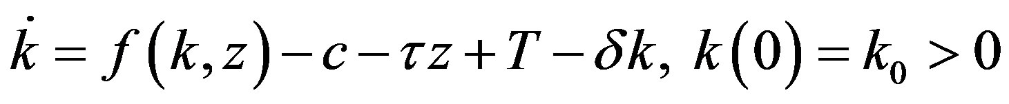
Since the use of polluting inputs in the production process may increase the amount of total polluting emissions in the environment,  , it is assumed that the government imposes a tax
  on the use of each unit of polluting inputs. Therefore, the law of accumulating capital stock reads:
 (2)
(2)
where  is consumption,
  is a lump-sum transfer from the government, and
  is a constant rate of capital depreciation.
Let the utility function  be increasing with respect to consumption,
  , but decreasing in the total amount of pollution,
 . Therefore, the representative household's optimal control problem needs to maximize
 (3)
(3)
where  indicates the household's discount factor, defined as
 (4)
(4)
subject to (2) and
 (5)
(5)
so that, the present value Hamiltonian becomes

where  and
and  represent the Lagrange multipliers of capital and discount, respectively.
The maximization problem requires the following first order necessary conditions:
 (6.1)
(6.1)
 (6.2)
(6.2)
 (6.3)
(6.3)
 (6.4)
(6.4)
joint with the transversality conditions
 (7.1)
(7.1)
 (7.2)
(7.2)
Second order sufficient conditions are also shown to hold. Therefore, the Hamiltonian is jointly strictly concave in  and
and  (see [24]).
Since, in equilibrium, both  and the government budget constraint
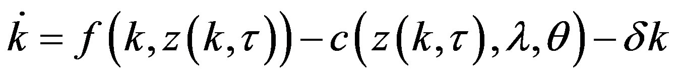
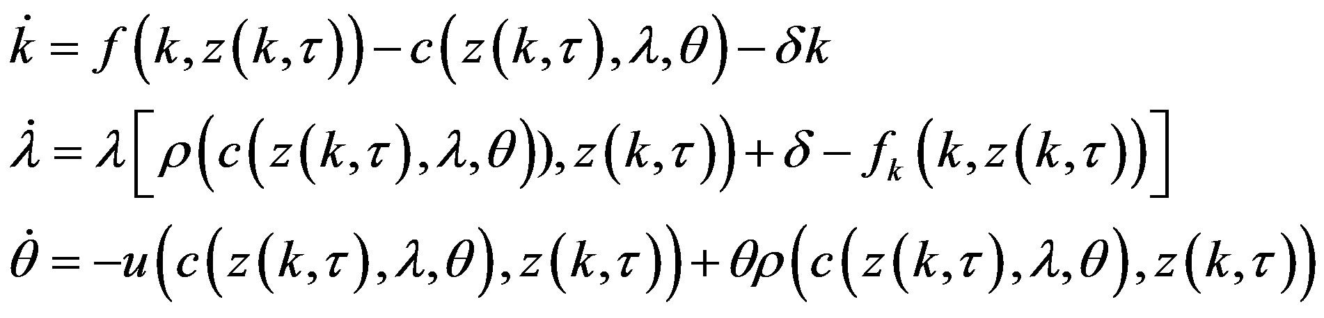
  hold, making log-derivatives of (6.1), and with a bit of mathematical manipulation, we easily derive the following three-dimensional autonomous system of first order differential equations


Specifically, system  becomes crucial for the purpose of the analysis we are going to deal with in the rest of the paper.
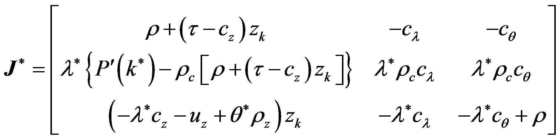
Let  be the Jacobian matrix associated with system
  given by:
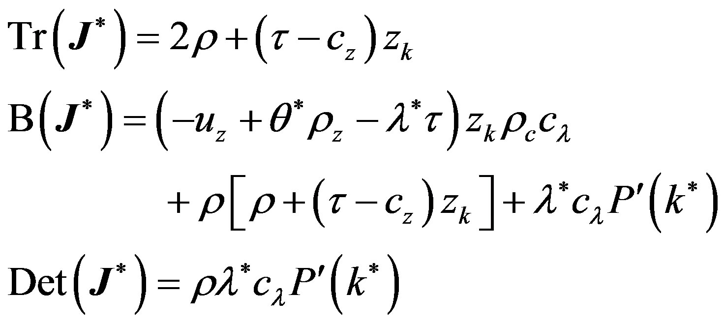
and let

be the characteristic polynomial of , where
  is the identity matrix. and
 ,
,  and
and  are the trace, sum of principal minors, and determinant to
 , respectively. Explicitly:
 (8)
(8)
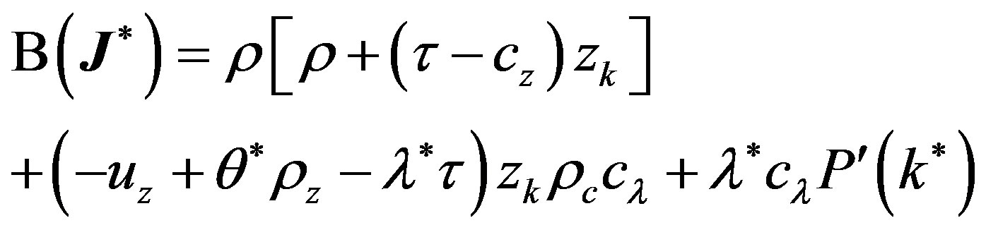 (9)
(9)
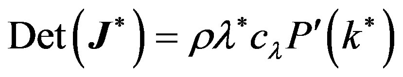 (10)
(10)
where
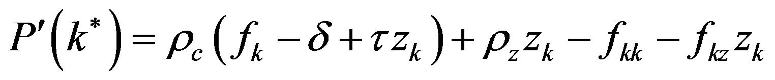 .
.
It is noteworthy to say that system  may exhibit many types of singularity situations, each of whom deserves particular attention, for different interesting consequences on the dynamic evolution of the economy being considered may eventually arise.
In [24] it is shown the possibility for local indeterminacy and the presence of multiple equilibria, depending on the characteristics of the discount rate function. Unfortunately, nothing is said on the long run properties of this economy outside the small neighborhood of the steady state. The aim of this paper is to show that, near the onset of a pitchfork-Hopf interaction, global indeterminacy can also arise, joint with the emergence of a quasi-periodic invariant torus dynamics in the original ℝ³ structure of the model. The next section is devoted to this end.
3. Global Indeterminacy and Invariant Torus
In what follows, we describe the systematic procedure to obtain the conditions for system  to undergo a pitchfork-Hopf interaction2. In this case, the linearization matrix,
  , at the origin exhibits one zero and a pair of pure imaginary eigenvalues. Interestingly, the possibility of a quasi-periodic toroidal motion, in some regions of the parameters space, assures that the dynamic motion of both predetermined
  and non-predetermined
  variables is regular across time, but it is never exactly repeating3. These property has a nice counterpart in terms of global indeterminacy, since for each initial value of the predetermined variable belonging to the three-dimensional compact set of points composing the interior of the torus, it is possible to show that there is 1) a continuum (in ℝ2) of possible initial values of the control variables (indeterminacy); and that 2) the solution is bound to stay in the vicinity of the fixed point (namely, it is an equilibrium); which possibly describes a phenomenon of global nature.
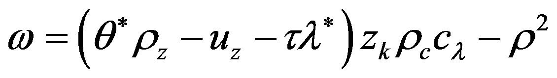
Lemma 1 Let  be the value that satisfies
 . Let furthermore
  be the value for which
 . Then, if
  and
and , the linearization matrix
  has a simple zero and a pair of pure imaginary eigenvalues,
  and
and , where
 . Straightforward computations show that
 ;
;
whereas,
 .
.
Proof To have a linearization matrix with a simple zero and a pair of pure imaginary eigenvalues in a ℝ3 ambient space, we need to make sure that both  and
and  vanish simultaneously.
  vanishes when
 . Solving (8), (9) and (10), we obtain the values in the Lemma.
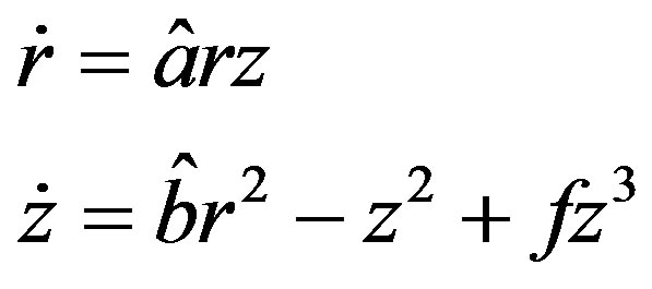
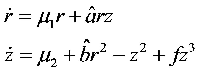
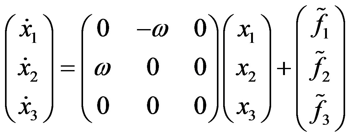
To ease the mathematical computation, we can transform system  into a more convenient Jordan normal form in cylindrical coordinates
 :
:
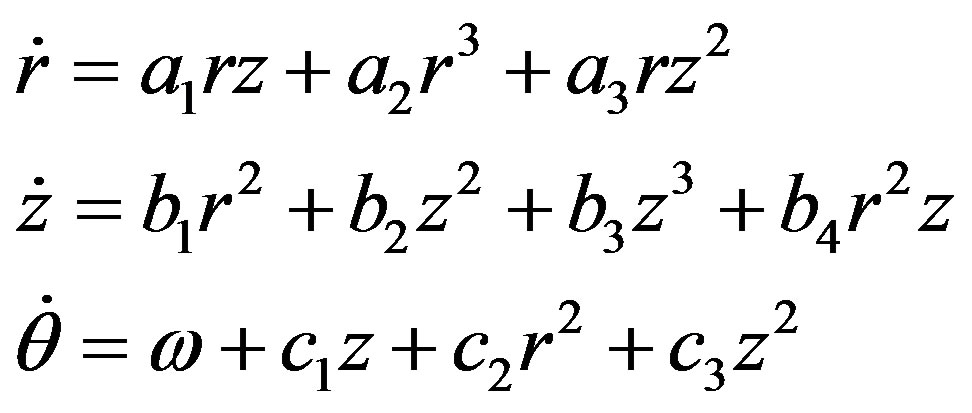 (11)
(11)
whose three-dimensional dynamics is topologically equivalent to the evolution of the original vector field in , when Lemma 1 is satisfied (see [25]).
In particular,  describes the amplitude of the limit cycle oscillations in the vicinity of the Hopf bifurcation. Noticeably, the first two equations are independent of
 , which describes a rotation around the
  -axis with almost constant angular velocity
 , for any
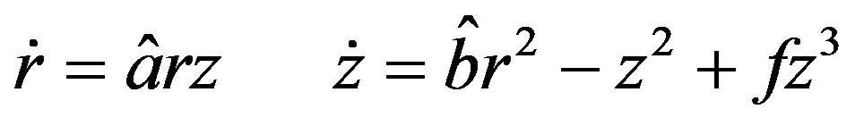
  small. Thus, we can restrain the analysis to a simpler two-dimensional vector field, which is often called a truncated amplitude system:
 (12)
(12)
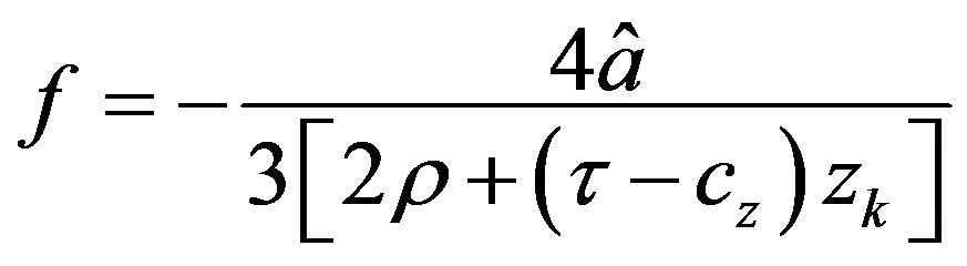
where
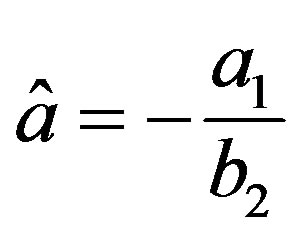 ,
,  , and
, and 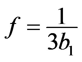 (see [25]).
A Versal deformation of the normal form in (12) can be found, and the bifurcation phenomenon can be studied in the neighborhood of the origin. This is not, in general, a trivial task. For our system we can show the following Proposition 1 The transverse family
 (13)
(13)
is a versal deformation of system (12), and is topologically equivalent to the original system, . Therefore, a non trivial equilibrium,
  , occurs at the pitchfork curve
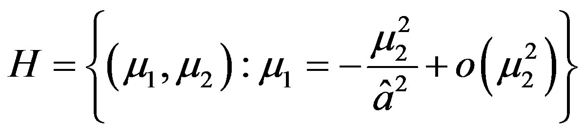
along which a cycle of small amplitude, and period , hopf-bifurcates from
 , which in fact corresponds to an invariant torus in the original ℝ3 vector field.
Proof See [26].
As clearly depicted in Figure 1, only for a limited set of parameters  located in region 2, a stable limit cycle appears in our model. InterestinglyRemark 1 if the planar system in (12) has a closed orbit, then the corresponding three-dimensional vector field in (11) has an invariant torus, which is encircling the
  -axis, with angular velocity
  (see, Figure 2).
We proceed now to locate more precisely the region of the parametric space implying the quasi-periodic dynamics described so far, and validate our findings with some numerical computations. To do so, we use the same set of parameters and the assumed explicit functions defined in [24], though we leave the chosen bifurcation parameters,  and
and , free to vary4.
Example 1 Set
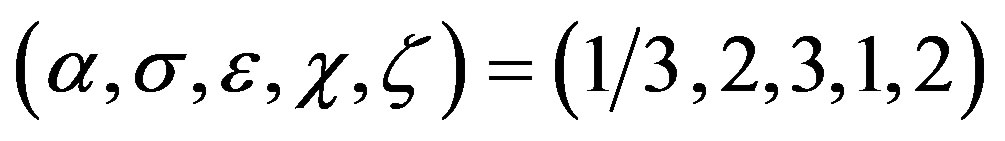
and . Then
 , with
 and
and .
.
A limit cycle emerges in the  phase space (see, Figure 3).
Example 2 Set

and . Then
 .
.
this choice implies
 and
and .
.
A limit cycle emerges in the  phase space (see, Figure 4).
Interestingly, we can notice that [24] finds that local indeterminacy occurs only when the condition  is verified, as in Example 1. However, the requirements for global indeterminacy are less stringent, since a pitchfork-Hopf bifurcation can emerge even when the above condition does not hold. In contrast to [24], we may say that, global indeterminacy is likely to occur even if the pollution tax rate is either too low or too high, both of them possibly giving rise to free-riding problems, and an unsustainable use of natural resources, at the expenses of the long-run consumption pattern of future generations.
Therefore, if the initial condition on capital is chosen in such a way that system  gives rise to a toroidal motion, then a continuum of equilibria can depart from a given initial condition of the predetermined variable. Since this continuum of equilibria exists beyond the region relevant for the linear approximation of the dynamics in the neighborhood of the steady state, the result implies indeterminacy of global nature [28].
Besides the result of global indeterminacy, the possibility that the model can exhibit toroidal motion is of great interest also because the decomposition of the dynamics into phase/amplitude equations allows us to better understand the nature of the cyclical behavior of an economy where the intertemporal consumption is influenced by the use of natural resources, and the long run properties of the equilibrium become totally unpredictable.
4. Concluding Remarks
This paper shows that the growth model with endogenous discounting proposed in [27] presents global indeterminacy of the equilibrium in the full onset of the original ℝ3 structure. In detail, a study of the properties of the steady state in the vicinity of a codimension 2 pitchfork—Hopf interaction, allows us to demonstrate that global indeterminacy can arise from plausible values of the parameters in correspondence of the emergence of a trapping region with an invariant torus quasi-periodic dynamics. The method innovates the literature in many aspects. First of all, it is the first time (to our knowledge) that a toroidal motion is shown to emerge in simple two-sector endogenous growth models of the standard type. Second, the form of indeterminacy of the equilibrium we detect is obtained in the full ℝ3 dimension, which implies that, given any initial value of the predetermined variable, there exists a continuum of initial values for the control (non-predetermined) variables in the ℝ2 submanifold.
Appendix
Given the following system
 (A.1)
(A.1)
the associated Jacobian matrix is

with
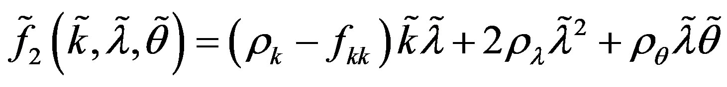
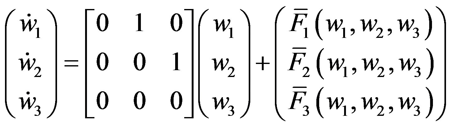
Consider a second-order Taylor expansion of the vector field in (A.1):
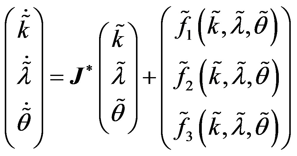 (A.2)
(A.2)
Where

Assume now that system (A.1) undergoes a triple-zero eigenvalue structure, which allows us to make the following change of coordinates
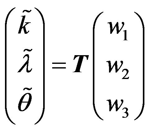 (A.3)
(A.3)
via an appropriate transformation matrix
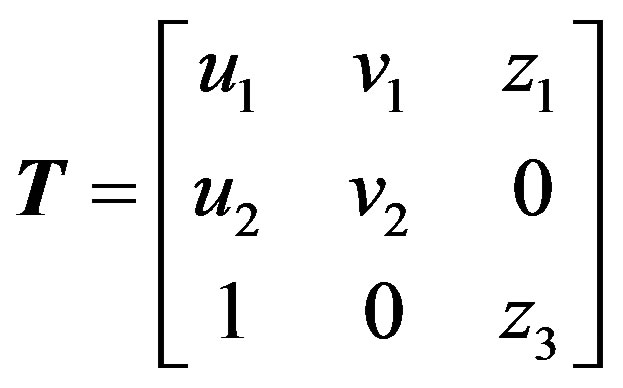 (A.4)
(A.4)
whose columns represent the eigenvectors associated to the triple-zero eigenvalues (see [28]).
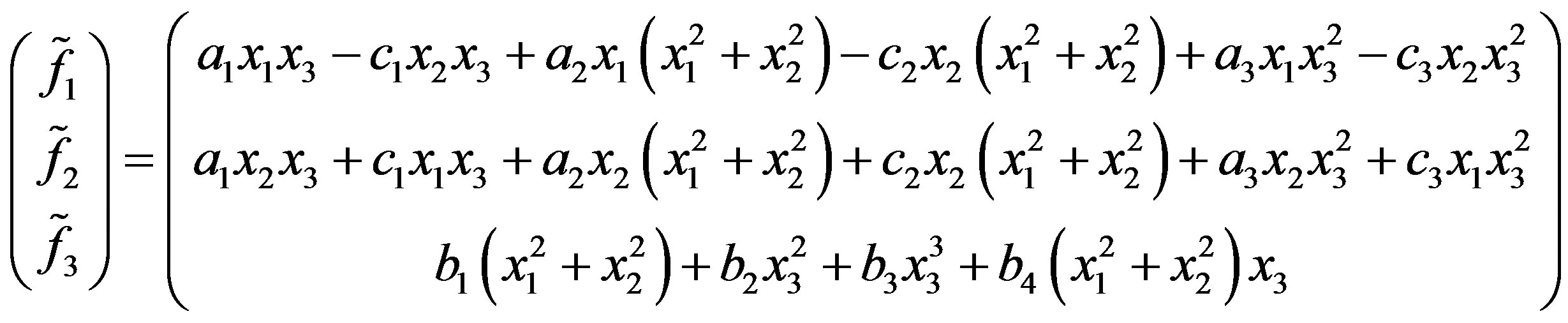
We are thus able to put (A.2) in a Jordan normal form
 (A.5)
(A.5)
where:
 (A.6)
(A.6)
with
 5.
5.
Let us repeat the same procedure of above, and introduce a second transformation matrix:
 (A.7)
(A.7)
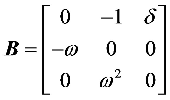
which allows us to put system (A.5) into the normal form suitable to describe the presence of one zero and a pair of pure imaginary eigenvalues:
 (A.8)
(A.8)
where
which can be easily transformed in cylindrical coordinates:
 (A.9)
(A.9)
given ,
,  ,
,  (see [25]).
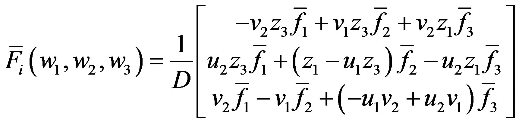
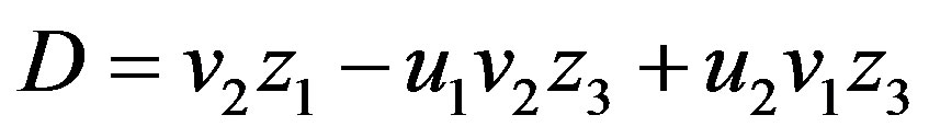
Following [29], the truncated-amplitude system is derived from (A.9), keeping :
:
 (A.10)
where
 ,
,  and
and
 .
.
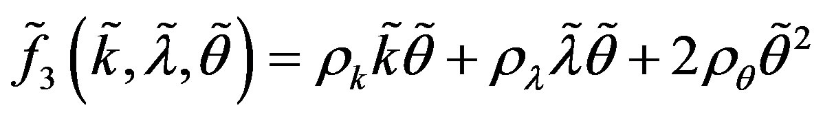
A candidate for versal deformation of (A.10) is then

with the following explicit values of
and

NOTES
2This is a codimension 2 bifurcation, since two parameters must be varied for such bifurcation to occur.
3This is also known as a codimension two Gavrilov-Guckenheimer bifurcation, where the interactions between a multiple equilibrium solution and the oscillatory pattern of each variable can lead to quasiperiodic motion in the vicinity of the singularity in the appropriate parametric set.
4To simplify the analysis, [24] has set . Our results are therefore more general and without restrictions.
5All further computations are available upon request.