Remarks on the Solution of Laplace’s Differential Equation and Fractional Differential Equation of That Type ()
1. Introduction
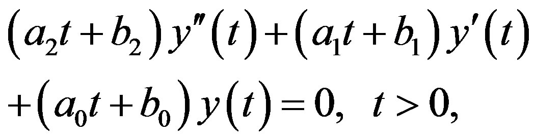
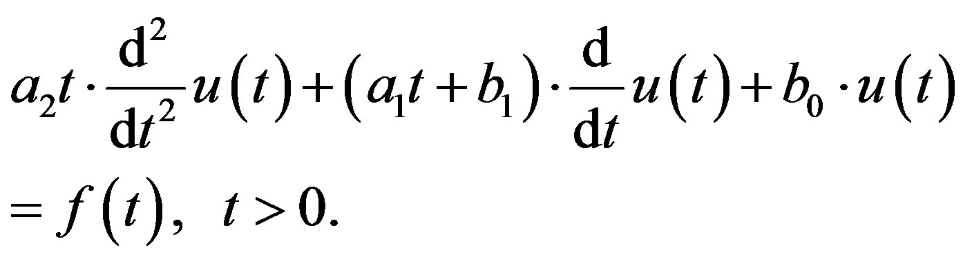
Yosida [1,2] discussed the solution of Laplace’s differential equation (DE), which is a linear DE with coefficients which are linear functions of the variable. The DE which he takes up is
 (1.1)
(1.1)
where  and
and  for
for  are constants. His discussion is based on Mikusiński’s operational calculus [3].
In our preceding papers [4,5], we discuss the initial-value problem of linear fractional differential equation (fDE) with constant coefficients, in terms of distribution theory. The formulation is given in the style of primitive operational calculus, solving a Volterra integral equation with the aid of Neumann series.
Yosida [1,2] studied the homogeneous Equation (1.1), where he gave only one of the solutions by that method. One of the purposes of the present paper is to give the recipe of obtaining the solution of the inhomogeneous equation as well as the homogeneous one, in the style of operational calculus in the framework of distribution theory. With the aid of that recipe, we show how the set of two solutions of the homogeneous equation is attained.
Another purpose of this paper is to discuss the solution of an fDE of the type of Laplace’s DE, which is a linear fDE with coefficients which are linear functions of the variable. In place of (1.1), we consider
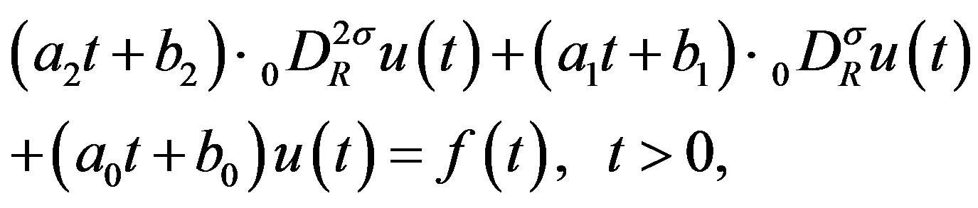 (1.2)
(1.2)
for  and
and . Here
  for
for 
is the Riemann-Liouville (R-L) fractional derivative defined in Section 2. We use  to denote the set of all real numbers, and
 . When
  is equal to an integer
 ,
, . When
 , (1.2) is the inhomogeneous DE for (1.1). We use
  to denote the set of all integers, and
 and
and  for
for
 satisfying
 . We use
  for
for , to denote the least integer that is not less than
 .
.
In Section 2, we prepare the definition of R-L fractional derivative and then explain how (1.2) is converted into a DE or an fDE of a distribution in distribution theory. A compact definition of distributions in the space  and their fractional integral and derivative are described in Appendix A. A proof of a lemma in Section 2 is given in Appendix B. After these preparation, a recipe is given to be used in solving a DE with the aid of operational culculus in Section 3. In this recipe, the solution is obtained only when
  and
and . When
 ,
,
 is also required. An explanation of this fact is given in Appendices C and D. In Section 4, we apply the recipe to the DE where
 , of which special one is Kummer’s DE. This is an example which Yosida [1,2] takes up. In Section 5, we apply the recipe to the fDE with
 , assuming
 .
.
The discussion is done in the style of our preceding papers [4,5].
2. Formulas
We use Heaviside’s step function, which we denote by . When
  is defined on
 ,
,  is assumed to be equal to
  when
when  and to
  when
when .
.
2.1. Riemann-Liouville Fractional Integral and Derivative
Let  be locally integrable on
 . We then define the R-L fractional integral
  of order
  by
by
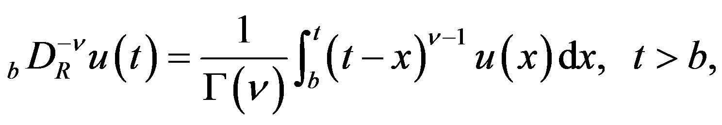 (2.1)
(2.1)
where  is the gamma function. The thus-defined
  is locally integrable on
 , and
, and 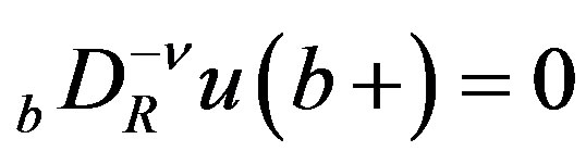 if
if .
.
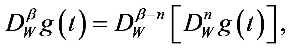
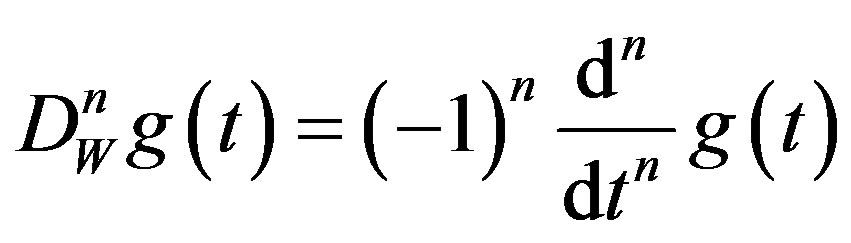
We define the R-L fractional derivative  of order
 , by
, by
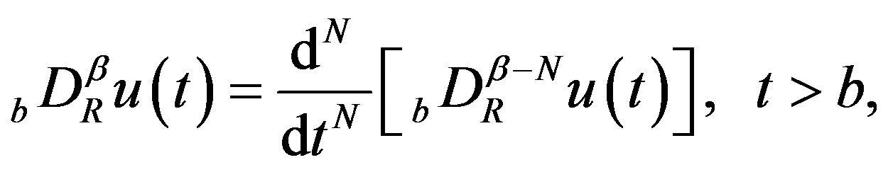 (2.2)
(2.2)
if it exists, where , and
, and 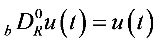 for
for .
.
We now assume that the following condition is satisfied.
Condition A  is locally integrable on
 , and there exists
  for
for , and
, and  for
for  are continuous and differentiable at
 , where
 . We then assume that there exists a finite value
 (2.3)
(2.3)
for every .
.
Because of this condition, the Taylor series expansion of  is given by
 (2.4)
(2.4)
where  is a function of
  as
as , so that
  as
as . By comparing (2.2)
and (2.4), we obtain .
.
2.2. Fractional Integral and Derivative of a Distribution
We consider distributions belonging to . When a function
  is locally integrable on
  and has a support bounded on the left, it belongs to
  and is called a regular distribution. The distributions in
  are called right-sided distributions.
A compact formal definition of a distribution in  and its fractional integral and derivative is given in Appendix A.
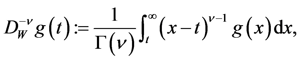
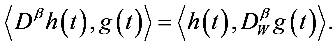
Let  be a regular distribution. Then
 for
for  is also a regular distribution, and distribution
  is defined by
 (2.5)
(2.5)
Let , and let
  be such a regular distribution that
  is continuous and differentiable on
 , for every
 . Then
  is defined by
 (2.6)
(2.6)
Let , for
, for  and
and
 , be continuous and differentiable on
 , for every
 . Then
 (2.7)
(2.7)
When  is a regular distribution,
  is defined for all
 .
.
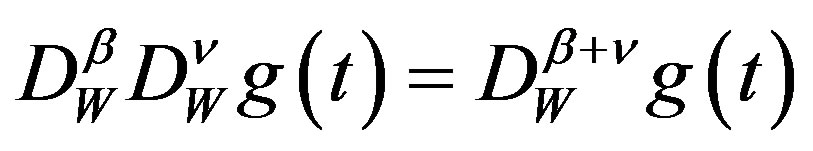
Lemma 1 For , the index law:
 (2.8)
(2.8)
is valid for every .
.
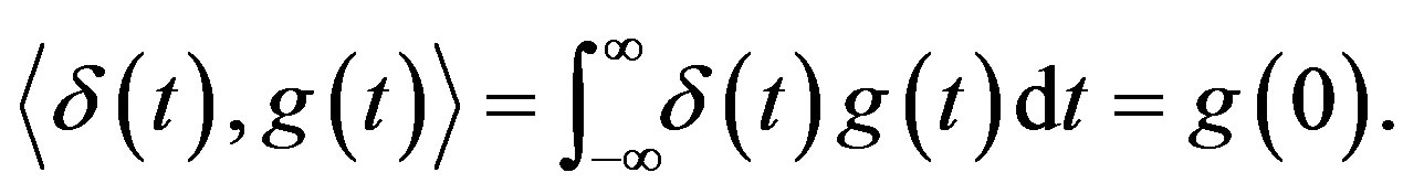
Dirac’s delta function  is the distribution defined by
 .
.
Lemma 2 Let  for
for . Then
 (2.9)
(2.9)
Proof By putting ,
,  , and
, and  in
in
(2.1), we obtain . By (2.5), we then have
 . By applying
  to this and using (2.6) and (2.8), we obtain (2.9).
We now adopt the following condition.
Condition B  and
and  are expressed as a linear combination of
  for
for .
.
Then  and
and  are expressed as
 (2.10)
Lemma 3 Let  exist for
 . Then the products
  and
and  belong to
 and they are related by
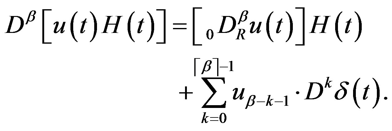 (2.11)
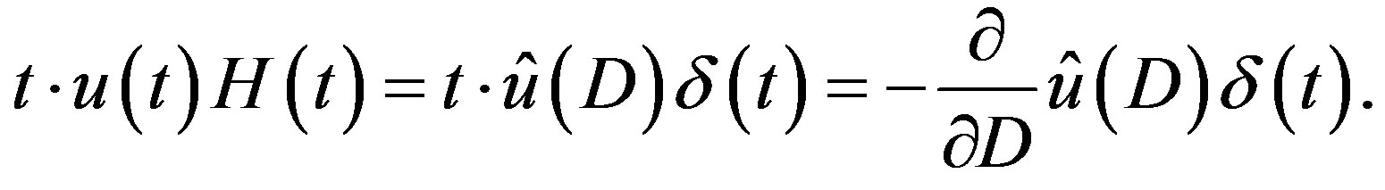
Proof We obtain (2.11) from (2.4) by multiplying  from the right and then applying
 . We first note
 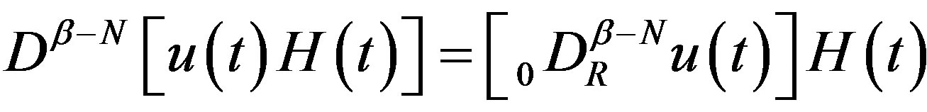 due to (2.5).
Applying  to this, we obtain the lefthand side of (2.11), and hence from the lefthand side of (2.4). We next note that
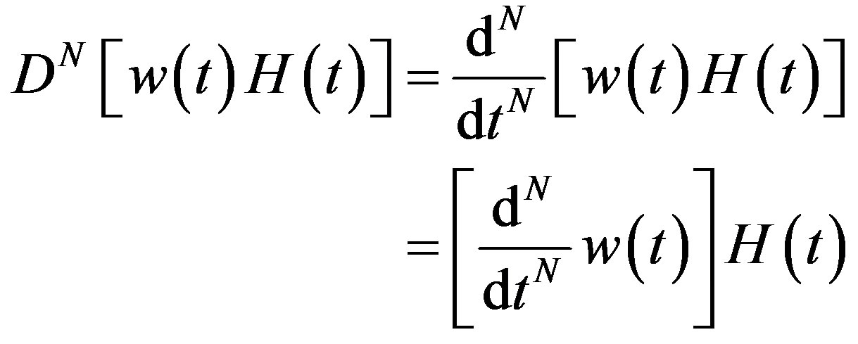
due to (2.6) and  as noted after
(2.4). Thus we obtain the first term on the righthand side of (2.11) from the last term of (2.4). As to the remaining terms, we only use (2.9). 
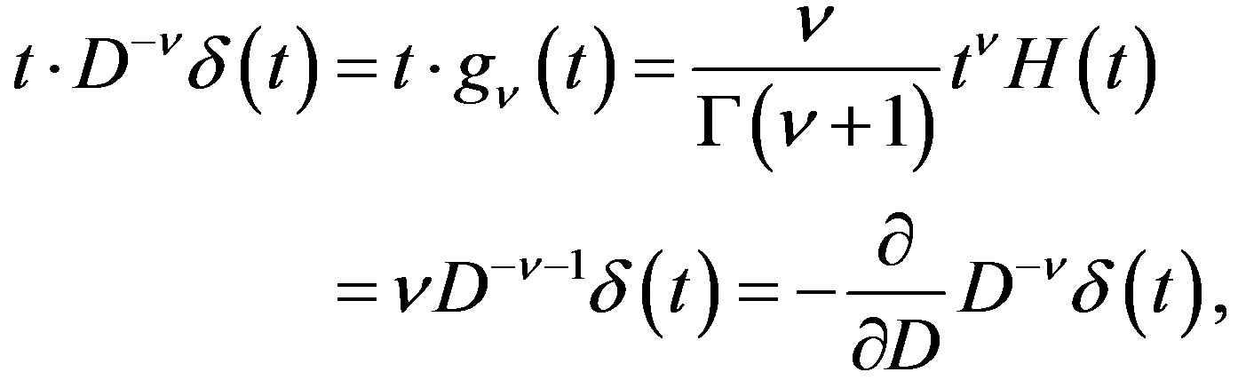
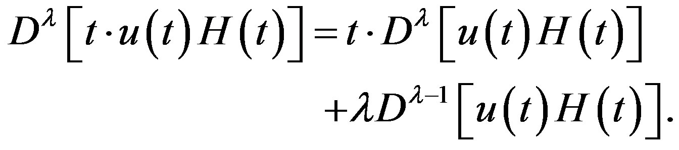
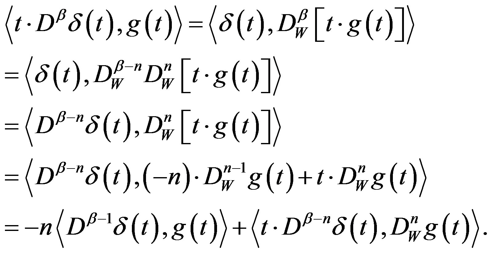
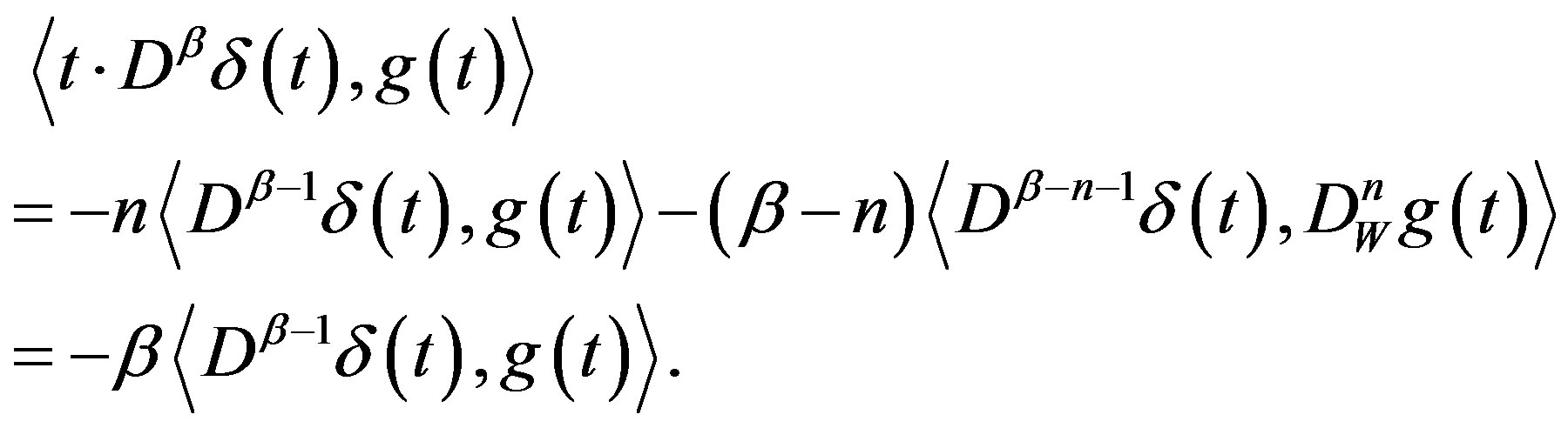
Lemma 4 Let . Then
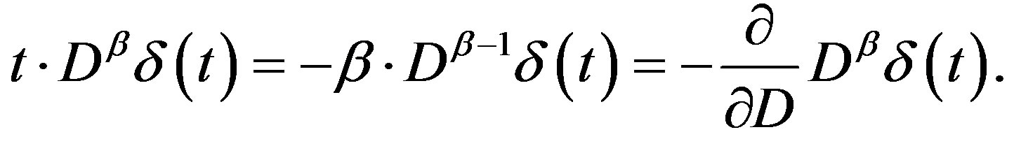 (2.12)
The last derivative with respect to  is taken regarding
  as a variable.
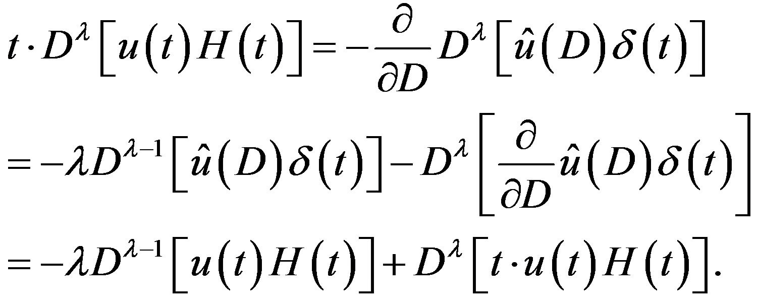
Proof of Lemma 4 for . Let
. Let ,
, . Then by (2.9), we have
by using (2.9) repeatedly. 
A proof of this lemma for  is given in Appendix B.
The following lemma is a consequence of this lemma.
Lemma 5 Let  satisfy Condition B. Then
 (2.13)
Lemma 6
 (2.14)
Proof By using (2.10) and (2.13), we obtain

3. Recipe of Solving Laplace’s DE and fDE of That Type
We now express the DE/fDE (1.2) to be solved, as follows:
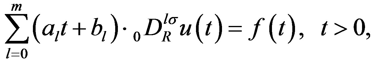 (3.1)
(3.1)
where  or
or , and
, and . In Sections 4 and 5, we study this DE for
  and this fDE for
 , respectively.
3.1. Deform to DE/fDE for Distribution
Using Lemma 3, we express (3.1) as
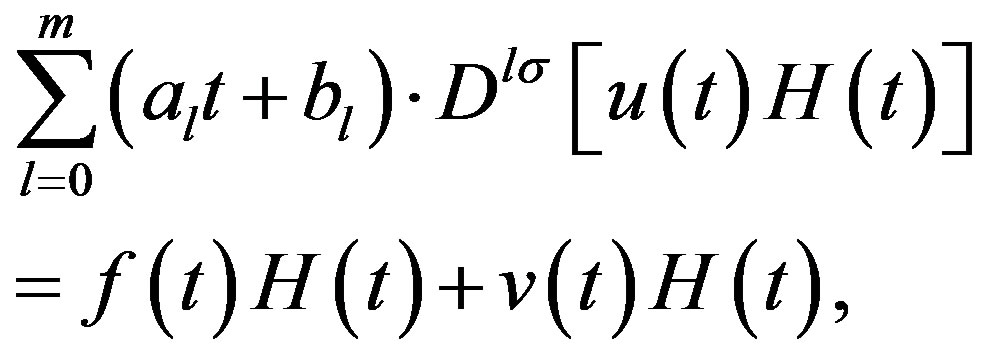 (3.2)
(3.2)
where
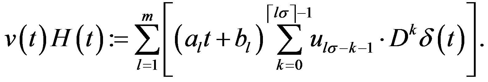 (3.3)
(3.3)
3.2. Solution via Operational Calculus
By using (2.10) and (2.13), we express (3.2) as
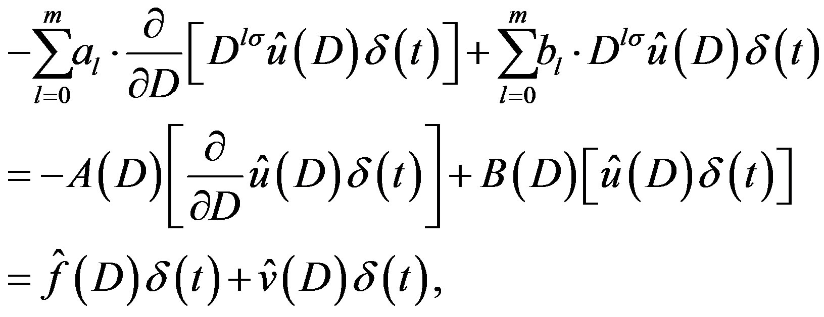 (3.4)
(3.4)
where
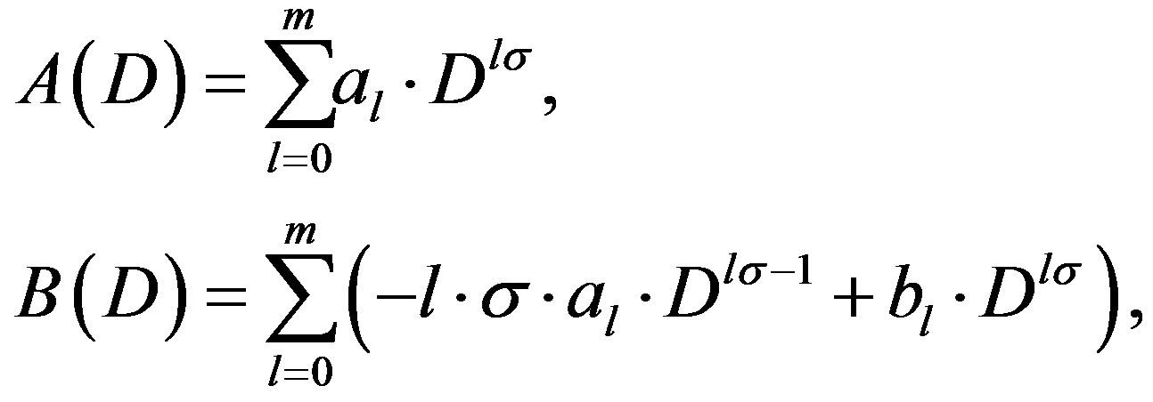 (3.5)
(3.5)
 (3.6)
(3.6)
In order to solve the Equation (3.4) for , we solve the following equation for function
  of real variable
 :
:
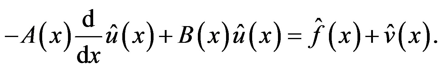 (3.7)
(3.7)
Lemma 7 The complementary solution (C-solution) of Equation (3.7) is given by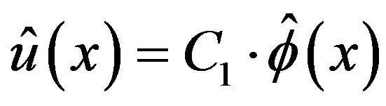 , where
  is an arbitrary constant and
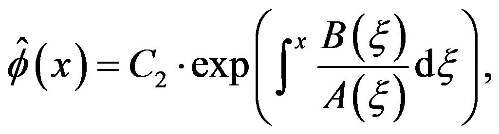 (3.8)
(3.8)
where the integral is the indefinite integral and  is any constant.
Lemma 8 Let  be the C-solution of (3.7), and let the particular solution (P-solution) of (3.7) be
  when the inhomogeneous part is
  for
for . Then
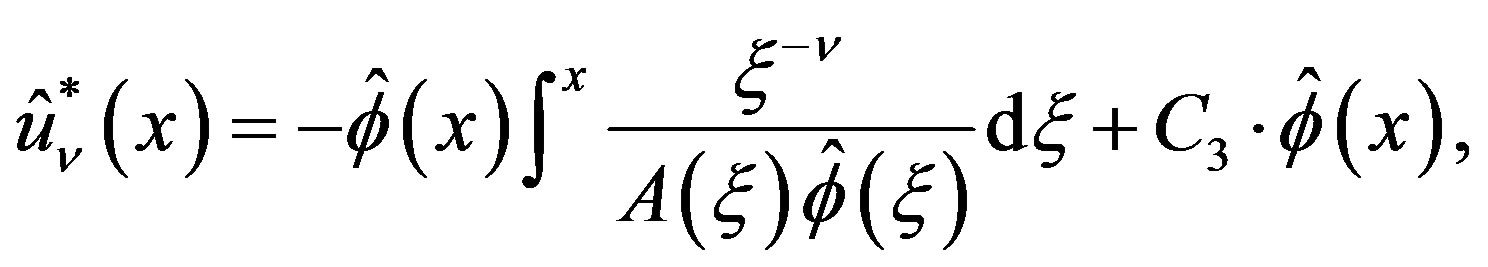 (3.9)
(3.9)
where  is any constant.
Since  satisfies Condition B and
  is given by (3.6), the P-solution
  of (3.7) is expressed as a linear combination of
  for
for  and
and  for
for .
.
From the solution  of (3.7),
  is obtained by substituting
  by
by . Then we confirm that (3.4) is satisfied by that
  applied to
 .
.
3.3. Neumann Series Expansion
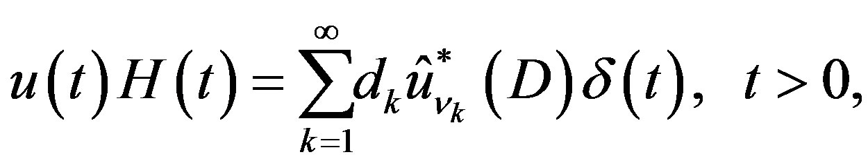
Finally the obtained expression of  is expanded into the sum of terms of negative powers of
 , and then we obtain the solution
  of (3.4). If the obtained
  is a linear combination of
  for
for ,
,  is converted to the solution
  of (3.2) by using (2.10) and (2.9). It becomes a solution
  of (3.1) for
 .
.
3.4. Recipe of Obtaining the Solution of (3.1)
1) We prepare the data:  by (2.10), and
 ,
,  and
and  by (3.5) and (3.6).
2) We obtain  by (3.8). If
 , the Csolution of (3.1) is given by
3) If  or
or , we obtain
  given by (3.9).
4) If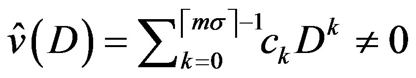 , the C-solution of (3.1) is given by
where  are constants.
5) If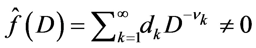 , the P-solution of (3.1)
is given by
where  and
and  are constants.
3.5. Solution of (3.1) from the Solution of (3.7)
In the above recipe, we first obtain the C-solution of (3.7), that is . It gives the C-solution
  of (3.4) and hence the C-solutions
  of (3.2) and
  of (3.1).
We next obtain the P-solution  of (3.7) when the inhomogeneous part is
  for
for . As noted above, the P-solutions
  of (3.7) for
  and for
 , are expressed as a linear combination of
  for
for  and of
  for
for , respectively. The sum of the P-solutions
  of (3.7) for
  and for
  gives the P-solution
  of (3.4) and hence the P-solution
  of (3.2). The C-solution
  of (3.1) comes from the C-solution of (3.7) and the P-solution of (3.7) for
 .
.
3.6. Remarks
When we obtain  at the end of Section 3.2, we must examine whether it is compatible with Condition B. We will find that if
  for
for , the obtained
  is not acceptable. Hence we have to solve the problem, assuming that
  for all
 .
.
When  and
and , we put
 . When
 and
and , we put
 . Discussion of this problem is given in Appendices C and D.
4. Laplace’s and Kummer’s DE
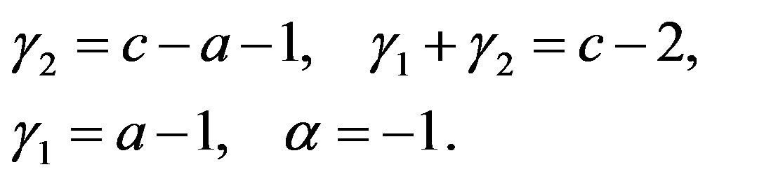
We now consider the case of ,
,  ,
,  ,
,  ,
,  and
and . Then (3.1) reduces to
 (4.1)
(4.1)
By (3.5) and (3.6),  ,
,  and
and  are
are
 (4.2)
(4.2)
 (4.3)
(4.3)
where .
.
4.1. Complementary Solution of (3.7), (3.4) and (3.2)
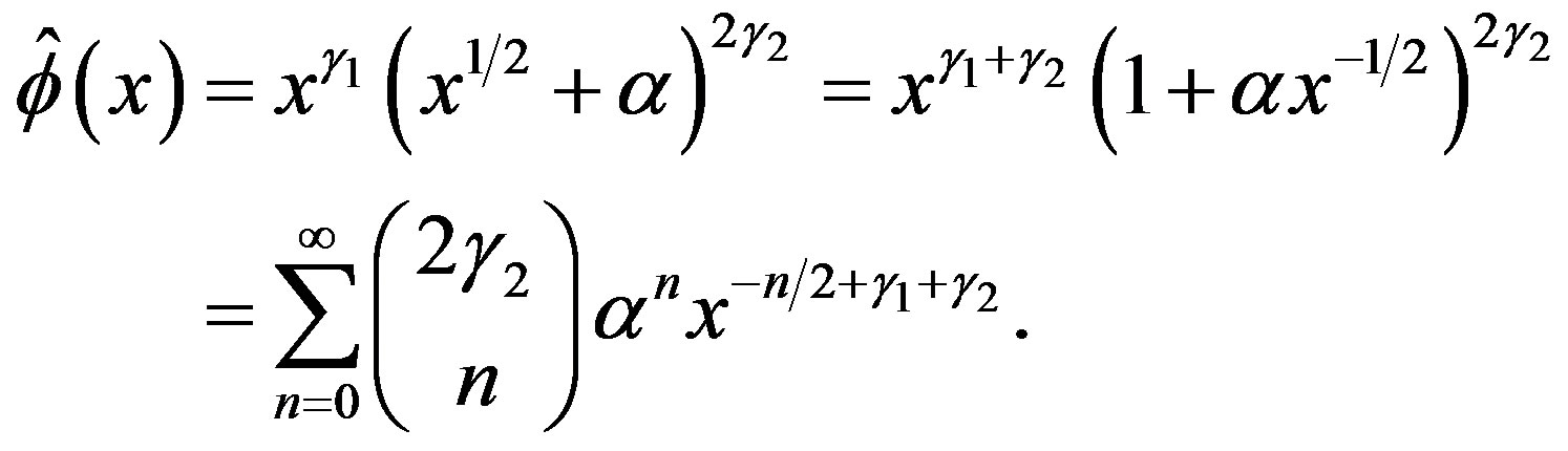
In order to obtain the C-solution  of (3.7) by using (3.8), we express
  as follows:
 (4.4)
(4.4)
where
 (4.5)
(4.5)
 is now expressed as
 .
.
By using (3.8), we obtain
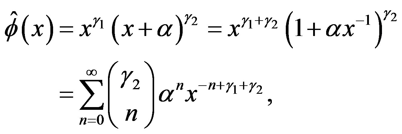 (4.6)
(4.6)
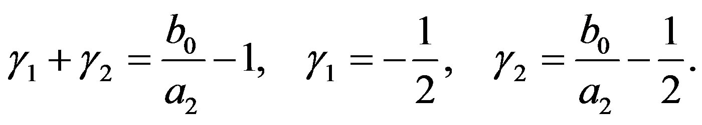
where 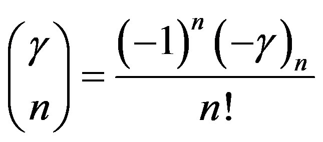 for
for  and
and 
are the binomial coefficients. Here 
for  and
and , and
, and .
.
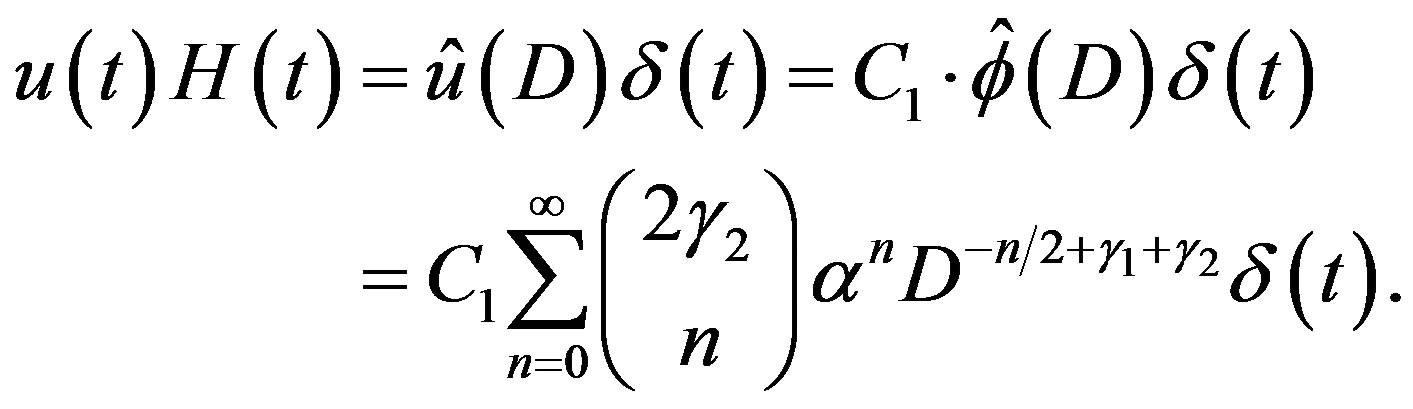
The C-solution of (3.4) is given by
 (4.7)
(4.7)
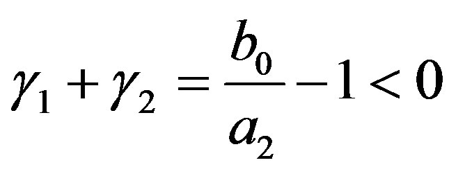
If , Condition B is satisfied. Then by using (2.9), we obtain the C-solution of (3.2):
 (4.8)
(4.8)
Remark 1 In [6,7], Kummer’s DE is given, which is equal to the DE (4.1) for ,
,  ,
,  and
and . In this case,
 (4.9)
(4.9)
We then confirm that the expression (4.8) agrees with one of the C-solutions of Kummer’s DE given in those books.
4.2. Particular Solution of (3.7)
We now obtain the P-solution of (3.7) when the inhomogeneous part is equal to  for
for .
.
When the C-solution of (3.7) is  given by (4.6), the P-solution of (3.7) is given by (3.9). By using (4.2) and (4.6), we obtain
 (4.10)
where
 (4.11)
Lemma 9  defined by (4.11) is expressed as
 (4.12)
Proof Equation (4.10) shows that the P-solution  of (3.7) is now expressed as
 (4.13)
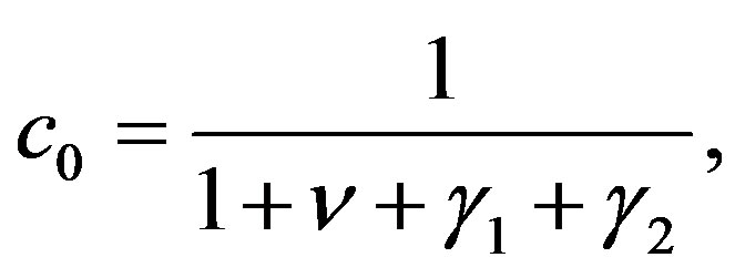
where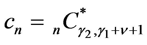 . Substituting this into (3.7), we obtain an equation which states that a power series of
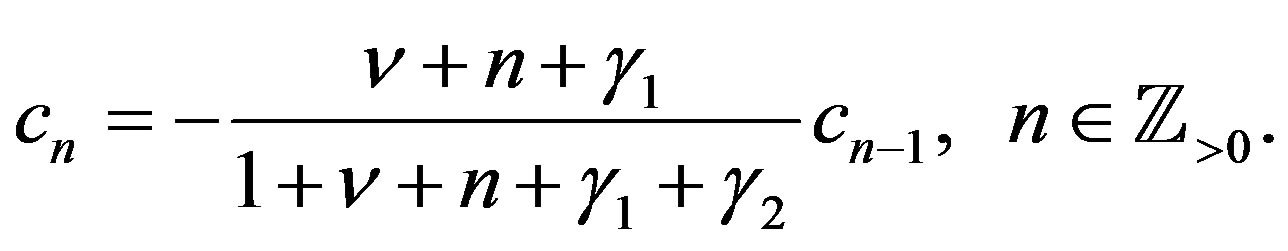
  is equal to 0. By the condition that the coefficient of every power must be 0, we obtain a recurrence equation for the coefficients
 :
:
 (4.14)
 (4.15)
By using this repeatedly, we have
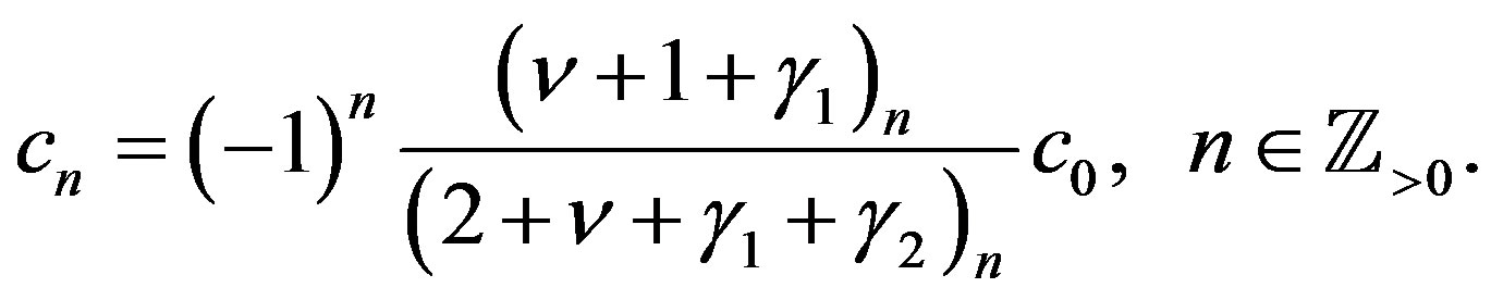 (4.16)
By comparing (4.10), (4.13) and (4.16), we obtain (4.12). 
4.3. Particular Solution of (3.2)
Equation (4.10) shows that if the inhomogeneous part is  for
for , the P-solution of (3.2) is given by
 (4.17)
By using (4.12) in (4.17), we obtain
 (4.18)
 (4.19)
4.4. Complementary Solution of (4.1)
By (4.3), . When the inhomogeneous part is
 , the P-solution of (3.7) is given by
 (4.20)
By using (4.18) for , we obtain
 (4.21)
Proposition 1 Let  and
and .
.
Then the complementary solution of (4.1), multiplied by , is given by the sum of the righthand sides of (4.8) and of (4.21).
Remark 2 As stated in Remark 1, in [6,7], the result for ,
,  ,
,  and
and , is given. In this case,
  and
and  are given in (4.9), and
 (4.22)
We then confirm that the set of (4.8) and (4.21) agrees with the set of two C-solutions of Kummer’s DE given in those books.
5. Solution of fDE (3.1) for 
In this section, we consider the case of ,
,  ,
,
 ,
,  ,
,  ,
,  and
and .
.
Then the Equation (3.1) to be solved is
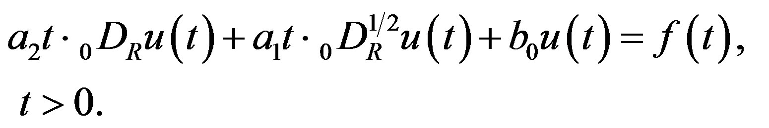 (5.1)
(5.1)
Then (3.5) and (3.6) are expressed as
 (5.2)
(5.2)
 (5.3)
(5.3)
where .
.
5.1. Complementary Solution of (3.7)
By using (5.2),  is expressed as
 (5.4)
(5.4)
where
 (5.5)
(5.5)
By (3.8), the C-solution  of (3.7) is given by
 (5.6)
(5.6)
5.2. Complementary Solution of (3.2) or (5.1)
The C-solution of (3.2) is given by
 (5.7)
(5.7)
By Condition B, we have to require
 .
.
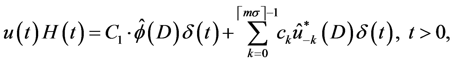
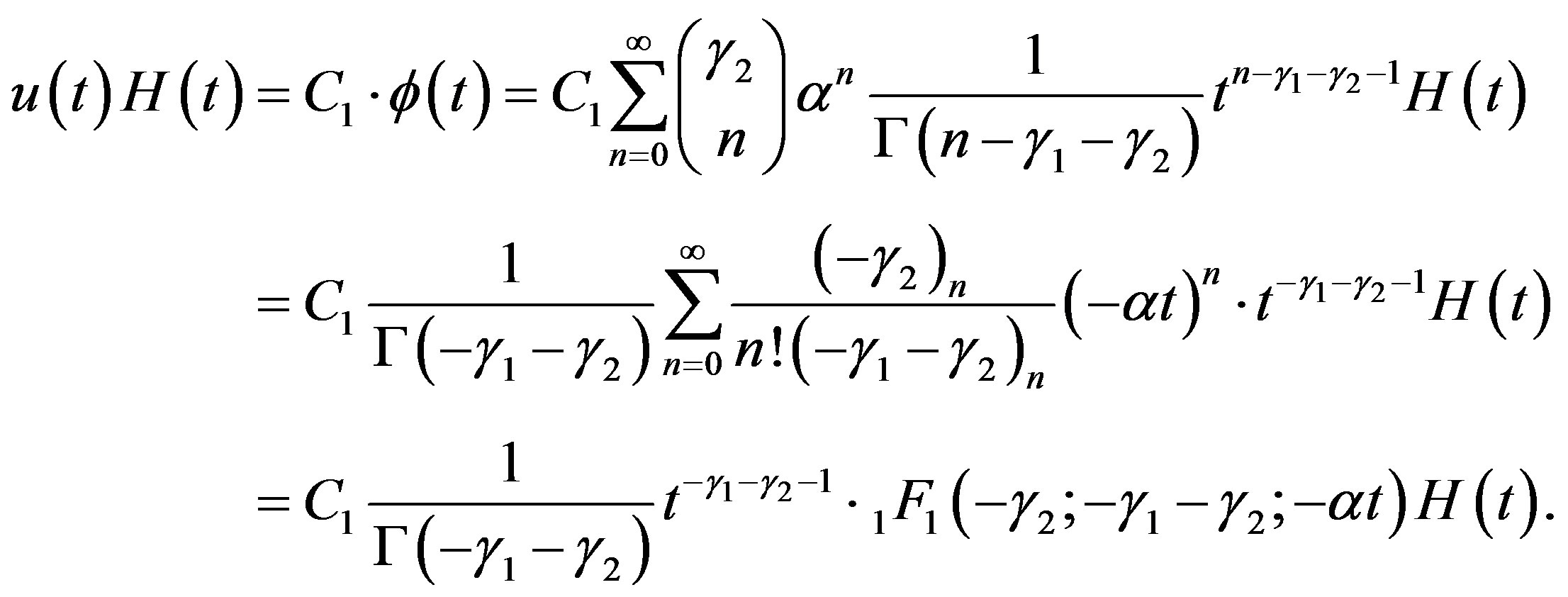
Then by using (2.9) in (5.7), we obtain
 (5.8)
(5.8)
The C-solution of (5.1) is equal to this for .
.
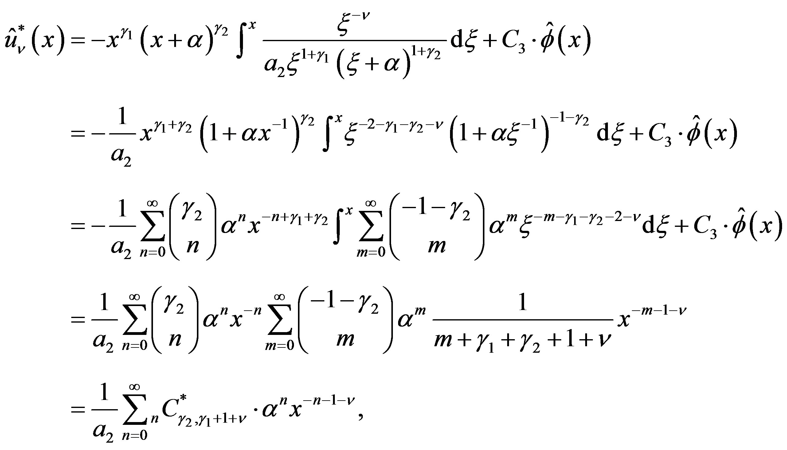
5.3. Particular Solution of (3.2) or (5.1)
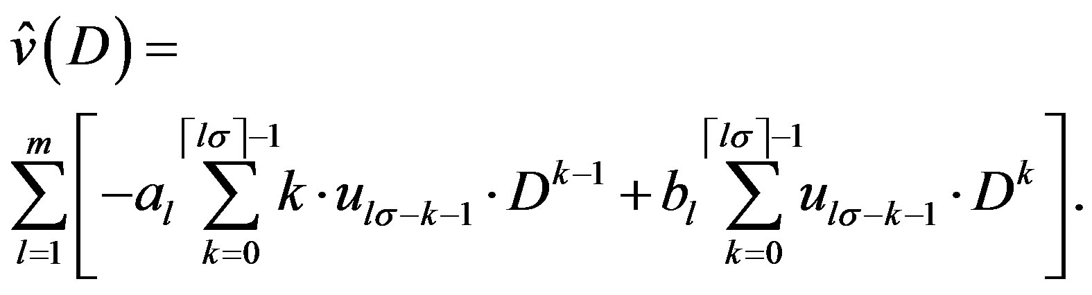
By using the expressions of  and
and  given by (5.2) and (5.6) in (3.9), we obtain the P-solution of (3.7) when the inhomogeneous part is
 :
:
 (5.9)
(5.9)
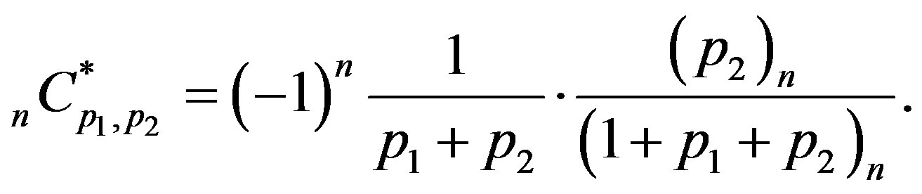
where  is defined by (4.11) and is given by (4.12).
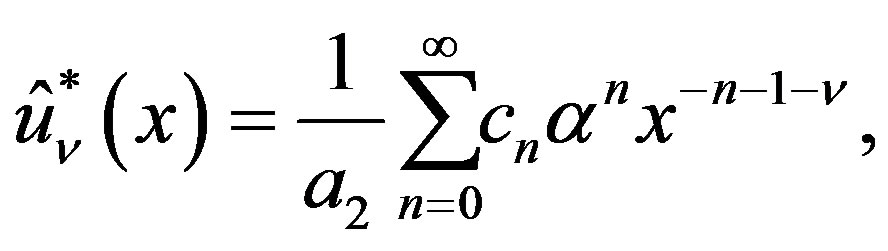
By using (4.12) in (5.9), we can show that if the inhomogeneous part is  for
for , the P-solution of (3.2) is given by
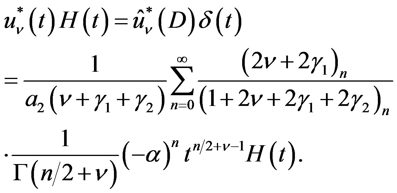 (5.10)
This  for
for  gives the P-solution of (5.1)when the inhomogeneous part is
  for
for .
.
Appendix A: Definition of a Distribution in  and Its Fractional Integral and Derivative
A right-sided distribution  is a functional for which a number
  is associated with all
 , where
  is the space of infinitely differentiable functions which is defined on
  and has a support bounded on the right.
A regular right-sided distribution  is a locally integrable function on
 , which has a support bounded on the left, and
  is given by
 (A.1)
(A.1)
Let . If
. If , the fractional integral
  is
is
 (A.2)
(A.2)
and if , the fractional derivative
  is given by
 (A.3)
(A.3)
where . We set
 , and
, and
for .
.
In this place, we can confirm that the index law
 (A.4)
(A.4)
is valid for every .
.
For a distribution ,
,  for
for  is defined by
 (A.5)
(A.5)
The index law (2.8) follows from (A.4) by (A.5).
Dirac’s delta function  is defined by
 , as stated just below Lemma 1, and hence
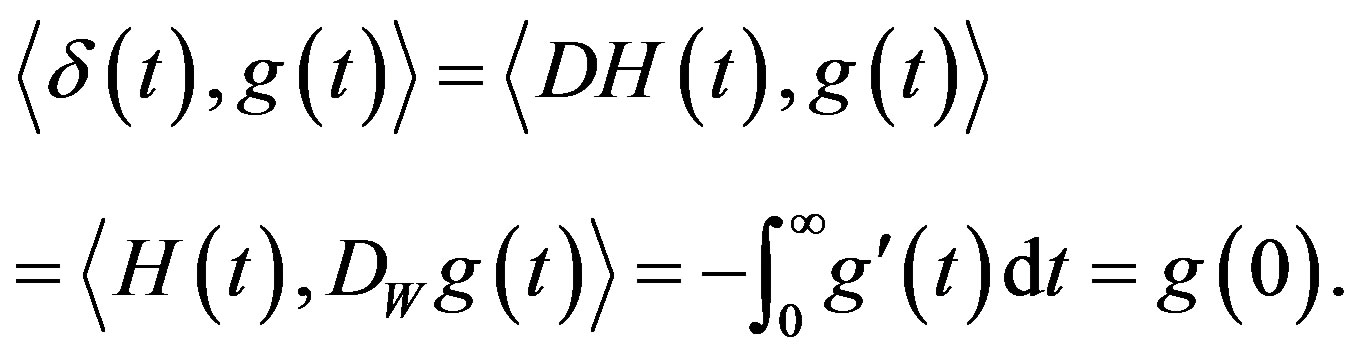 (A.6)
(A.6)
It is customary to use the notation:
 (A.7)
(A.7)
Let  and
and . Then
  is defined by
 (A.8)
(A.8)
Appendix B: Proof of Lemma 4 for 
Here we give a proof of Lemma 4 for , with the aid of notations explained in Appendix A.
Let ,
,  and
and . Then
Using Lemma 4 for  in the last member, we obtain
Formula (2.12) for  follows from this.
Appendix C: Solution of Laplace’s DE (3.1) for 
We now consider the DE (3.1) for  and
and . Then (3.5) and (3.6) are expressed as
 (C.1)
(C.1)
 (C.2)
(C.2)
 (C.3)
(C.3)
where
 (C.4)
(C.4)
In solving (3.7), we express  as
as
 (C.5)
(C.5)
where  and
and  are constants. In Section 4.1, we assume that
  and obtain the C-solution given by (4.8) which satisfies Condition B. In the presence of the first term on the righthand side of (C.5), we will see that we cannot obtain a solution satisfying Condition B. Hence we have to assume
 .
.
Appendix D: Solution of fDE (3.1) for 
In this section, we consider the fDE (3.1) for 
and . Then (3.5) and (3.6) are expressed as
 (D.1)
(D.1)
 (D.2)
(D.2)
 (D.3)
(D.3)
where  are given by (C.4).
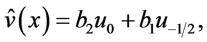
In solving (3.7), we express  as
as
 (D.4)
(D.4)
where  and
and  are constants. In Section 5.2, we assume that
  and obtain the C-solution given by (5.8) which satisfies Condition B. In the presence of the first two terms on the righthand side of (D.4), we will see that we cannot obtain a solution satisfying Condition B. Hence we have to assume
 .
.