Correlation and Prediction of the Solubility of Solid Solutes in Chemically Diverse Supercritical Fluids Based on the Expanded Liquid Theory ()
1. Introduction
During the past few years, widespread attention has been focused on supercritical fluids due to their potential application in extraction processes in foods processing, pharmaceuticals, flavors, chemicals and petroleum industries. The main advantages of supercritical fluid extraction over conventional extraction methods include increased speed, easy solvent separation and better recovery, and reduction in both solvent usage and solvent waste generation. The solubility of a solute in a supercritical fluid is perhaps the most important thermophysical property that must be determined and modeled for an efficient design of any extraction procedure based on supercritical solvents. The determination of solubilities of a wide variety of solids and liquids of low volatility in supercritical fluids has received considerable attention in recent years. However, despite the vital importance of the solubility data of different compounds from chemical, biochemical, pharmaceutical and industrial points of view, there is still a lack of fundamental solubility and mass-transfer data available in the literature to facilitate the development of commercial-scale processes. Since the experimental determination of the solubilities of various solutes in supercritical fluids at each operating condition is tedious, time-consuming and not reported in literatures, there is a considerable interest in mathematical models that can accurately predict the solubilities of solid solutes in supercritical fluids [1]. Therefore it is essential to have a model that not only can accurately correlate but also predict phase equilibrium properties. Some of the models that have been used for correlating solubility data can be classified in two classes, equations of state based models (EOS) [2] and empirical models [3,4]. EOS based models require the prior knowledge of a certain number of parameters such as the critical properties (temperature and pressure), acentric factor and the sublimation pressure of the solid solute. These parameters are not available and specifically for many high molecular weight compounds and are calculated using group contribution methods, which could lead to solubility error prediction. Due to the lack of information on these properties, empirical models are often used for the correlation of experimental solubility data. These models are known as density-based models and consist of equations that contain constants that are empirically adjusted for each compound. Although simple, these models rely much on the knowledge of the thermodynamic behaviour of the supercritical solvent rather than of the solute, and are mostly capable of correlating rather than predicting the solubility. They are used for quantitative determination of the solute solubility in supercritical phase at equilibrium, and do not provide qualitative information about the solute-solvent interaction.
In a previous presentation [5], we have adopted a methodology for the correlation and the prediction of the solubility of 10 aromatic pollutants in the supercritical carbon dioxide. In this work we present an extension of the methodology to the solubility of other solids with different functional groups in different supercritical fluids namely carbon dioxide, ethylene and ethane. The methodology is based on the expanded liquid model theory [6,7] which does not require the knowledge of the solute critical properties and sublimation pressure. In this case the supercritical phase is considered as an expanded liquid and is modeled using excess Gibbs energy models such as Margules, Van Laar, and local composition based models i.e. Wilson, NRTL and UNIQUAC. In this study we focus on the use of the UNIQUAC model that has been widely used in modeling vapour-liquid and liquid-liquid equilibria data. This model does not only take the size and nature of the molecules into consideration, but also accounts for the strength of solute-solvent intermolecular forces. And because the primary concentration variable is the surface fraction rather than mole fraction, the UNIQUAC model is applicable to solutions containing small or large molecules, including polymers. To assess the correlative and predictive capabilities of this model, a database is built by consisting of the experimental solubility data of 33 binary systems solid-super-critical fluid where solid solutes have different functional groups.
2. Model Development
In the supercritical state, a fluid has a high density when compared with a gas. In fact, the density of a supercritical fluid is closer to that of a liquid than that of a gas. Consequently, in theoretical treatments the supercritical fluid phase can be treated approximately as an expanded liquid. This allows the phase equilibria between the solute and the supercritical fluid to be represented thermodynamically by solid-liquid equilibrium relations and conventional activity coefficients. To estimate the solid solubility in the supercritical phase, the knowledge of the activity coefficients are required. These coefficients are determined from the knowledge of the component fugacities, thus when the equilibrium of the pure solid and the supercritical phase is reached, we have:
 (1)
(1)
 is the fugacity of the solute in the solid phase considered as pure solid and equal to
  because the solubility of supercritical fluid (SCF) in the solid phase is considered to be negligibly small. The
  is the fugacity of the solid solute in the supercritical phase and is equal to:
 (2)
(2)
Equation (1) could be written as follows:
 (3)
(3)
where ,
,  and
and  are the activity coefficient, the solid solubility represented in mole fraction and the fugacity of the pure solid solute in the expanded liquid phase respectively. According to Prausnitz et al. [8], we have:
 (4)
(4)
Prausnitz et al. [8] stated that, to a fair approximation, the heat capacity terms can be neglected. Equations (3) and (4) then combined to yield an expression for the solute solubility:
 (5)
(5)
 is the enthalpy of fusion, Tm is the melting point temperature of the solid solute. Since the solid solubility in the supercritical phase is very small, we can assume to be at infinite dilution condition. Consequently, the activity coefficient of the solid solute is the one at infinite dilution and the density of the solution is that of the pure solvent. Thus Equation (5) becomes:
 (6)
(6)
The activity coefficient of the solid solute at infinite dilution  was calculated using the UNIQUAC model which consists of two parts, a combinatorial part
  that attempts to describe the dominant entropic contribution, and a residual part
  that is due primarily to intermolecular forces that are responsible for the enthalpy of mixing. The combinatorial part is determined only by the composition and by the sizes and shapes of the molecules; it requires only pure-component data. The residual part, however, depends also on intermolecular forces; the two adjustable binary parameters a12 and a21, therefore, appear only in the residual part [8]:
 (7)
(7)
 (8)
(8)
Here q and r are the surface area and volume parameters; z is the coordination number that is usually taken equal to 10. The residual part at infinite dilution is given by the following equation [8]:
 (9)
(9)
where
 (10a)
(10a)
and
 (10b)
(10b)
 and
and  are characteristic energies and are related to the interaction parameters
  and
and  through Equation (10). Finally combining Equations (9) and (10) leads to:
 (11)
(11)
Equation (11) could be written in reduced form by introducing the reduced temperature, thus we obtain:
 (12)
(12)
With  and
and , Tc is the solvent critical temperature.
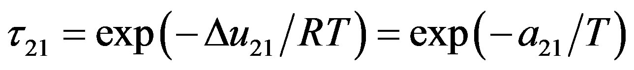
The binary interaction parameters  and
and  are related to the energy of interaction between the solid solute and the solvent in the supercritical phase, and cannot be kept constant and specifically at high pressure conditions. Therefore to take into account the pressure and temperature effects, these parameters are assumed to be density dependent and were fitted to the following equations:
 (13a)
(13a)
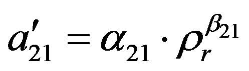 (13b)
(13b)
 is the reduced density of the solvent equal to ρ/ρc1 where ρc1 is its critical density,
  ,
,  ,
,  and
and  are the regressed parameters of the model.
3. Database Compilation
By considering 33 system solid-SC fluid, an exhaustive solutes solubility database consisting of more than 2218 solubility data in supercritical fluids is built-up for the elaboration and validation of the proposed model. It is acknowledged that the systems studied do not include all the data available but should be sufficient to provide a thorough testing of the potential of Equations (6) to 13(b). The density of supercritical fluid solvents used in this work, is estimated using the Span and Wagner equation of state [10] when they are not reported in the solubility data sources, the physical properties of the solvents are given in Table 1. Table 2 show the solutes and their thermodynamic properties obtained from literature used in this study. Description of the database is given in Table 3 which lists the binary systems used together with the number of solubility data points, and the lower and upper limits of the operating conditions, solubility and the references. Detailed information about all the complete references from which experimental solubility data are taken are provided in Table 4.
4. Solutes Solubility Correlation
The surface area and volume parameters are calculated as the sum of the group volume and area parameters (R and Q) given by the UNIFAC group specifications [8]. These parameters and properties listed in Table 2, together with those of different fluids listed in Table 1 are used to calculate the combinatorial part of the activity coefficient from Equation (8). In other hand, Equation (12) is used to calculate the residual part of the solid solute activity coefficient. Thermodynamic properties of the solid solute listed in Table 2 are used together with Equations (7), (8), and (12) to estimate the solubility y2 using Equation (6). The interaction parameters  and
and  are then regressed according to Equations 13(a) and 13(b). The best regression is based on minimizing the error between the regressed and experimental solubility data. The objective function used minimizes the sum of average absolute relative deviation (AARD) according to Equation (14):
 (14)
(14)
where N is the number of experimental solubility data of each solute.

Table 1. Solvents physical properties.
aFrom reference [8], bFrom reference [9].

Table 2. Solute species properties.
5. Solutes Solubility Prediction
In order to evaluate the predictive ability of the proposed model, the solubility data for each considered component are split with specific tool in two sets. The first data set is the training set on which the minimization routine is performed and the interaction parameters are regressed. This data set contains 70% of the data randomly picked up from the experimental solubility data for each component. The second data set, namely the test set, contains the remaining 30% data and is intended for testing the generalized capabilities of the UNIQUAC model. The interaction parameters have been regressed using the training solubility data set, and then used directly to predict the solid solubility y2 using the test data set. The predictive ability of the model is then assessed by comparing the obtained AARD values for each data set and so for each component.


Table 4. References for solubility data.
6. Results and Discussion
6.1. Solubility Data Correlation
The analysis of the correlation model results is done through statistical calculations. Table 5 provides the quantitative results of the regression for the UNIQUAC model. The AARD is included for each binary system and is listed together with the adjustable parameters values. Each component parameters are obtained by fitting them on its own solubility data available in the database. For all investigated systems the resultant AARD values are lower than 20% (except for the system phenol-CO2). The model achieves an overall AARD of 12.16 on a range of 2.8 to 29.7. These results are indicative of a good correlation performance of the proposed model and also show that the calculated solubility data are in good agreement with the experimental ones.
In order to compare more clearly, the experimental data and correlated data in this work are compared in Figures 1-3 with naphthalene in SC CO2 at T = 308 K,

Figure 1. Experimental and correlated solubility versus reduced density of naphthalene-CO2 system at 308 K.

Figure 2. Experimental and correlated solubility versus reduced density of naphthalene-ethylene system at 298 K.

Figure 3. Experimental and correlated solubility versus reduced density of naphthalene-ethane system at 308 K.
naphthalene in SC ethylene at T = 298 K, and naphthalene in SC ethane at T = 308 K respectively. These systems are arbitrarily taken from the database for illustration. From the figures, we see that it is good accordance with experimental and calculated ones, and the precision of the model in this work is very acceptable.
6.2. Comparison with Literature
We have considered for the comparison some literature models that account for effect of the system conditions (temperature and pressure) in addition to the physical properties as sublimation pressure of the solute through their introduction of the enhancement factor and a model based on a modified equation of state.
6.2.1. Wang and Tavlarides Model
Based on a dilute solution theory, Wang and Tavlarides [22] proposed the following model:
 (15)
(15)
where Z is the compressibility factor, E is the enhancement factor that is defined as the enhancement of actual mole fraction solubility of the solid solute y2 over the solubility in an ideal gas , i.e.,
  .
. 
and P are the sublimation vapor pressure and total pressure respectively. By introducing reduced variables, the dimensionless form of Equation (15) is given by:
 (16)
(16)
where ;
; .
.
6.2.2. Méndez-Santiago and Teja Models
Based on the theory of dilute solutions, Méndez-Santiago and Teja [23] began with the Henry’s constant and presented a simple linear relationship for the solubility of solids in supercritical fluids as given below:
 (17)
(17)
To apply the model to compounds whose sublimation vapor pressure is unknown, a Clausius-Clapeyron-type expression for the sublimation pressure  and
and 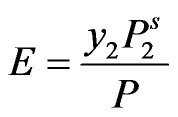 are substituted into Equation (17) resulting in the following expression:
 (18)
(18)
The dimensionless form of Equations (17) and (18) are given bellow [4]:
 (19)
(19)
where:
 ;
; 
 (20)
(20)
where:
 ;
;  ;
;  ;
; 
The linear behavior of Equation (17) is well observed in the range (0.5 - 2) of reduced density of the super-


Table 5. Regression parameters and average deviation of the model.
critical solvent [23], for this reason we have omitted from the database all data points over this range of density (see Table 3).
6.2.3. Schmitt and Reid Model
By the assumption that: the system pressure is much greater than the sublimation pressure of the solute, that the solute is incompressible, and that no solvent is dissolving in the solid phase, the solubilities of solids in supercritical solvents are usually correlated with the equation bellow [24]:
 (21)
(21)
 is the molar volume of the solute (Table 2), the fugacity coefficient of the solute in the supercritical phase
  is determined from an equation of state applicable to the solute-solvent mixture. The Peng-Robinson equation of state, i.e. PR-EOS is a commonly used approach for correlating solubility in supercritical fluids.
Schmitt and Reid [24] used this equation of state for modeling solid solubilities in supercritical fluids but not in the traditional manner due to the lack of the critical properties values and the low accuracy of their estimation. In fact they eliminated the binary interaction parameter and they assumed the solid solute parameters “a2” and “b2” independent of temperature and they eliminated the terms with y2 in the combining and mixing rules since the values of y2 were sufficiently small. Thus they propose the simplified equation bellow for the fugacity coefficient:
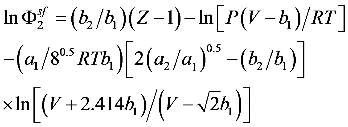 (22)
(22)
For the supercritical solvent, the parameters a1 and b1 are given by:


Equation (21) becomes,
 (23)
(23)
The experimental solubility data are regressed by using Equation (23) to determine the parameters of the solute a2 and b2 for each binary system considered. These parameters are expressed in Pa (m3/mol)2 and m3/mol respectively. The Equation (23) is dimensionally consistent and already dimensionless, but the parameters “a2” and “b2” are not. For comparison on the same basis the dimensionless parameters are as follow:
 and
and 
6.3. Analysis and Discussion
As mentioned in the previous section, the three first correlations used for comparison require the knowledge of the sublimation pressure. Table 6 gives the coefficients for the estimation of the sublimation pressure of the different solutes taken from literature and the temperature range of applicability.
To compare all the correlations on the same basis, the average absolute relative deviation (AARD) is determined for each system’s solute using each model. Table 7 display the parameters of the comparison models and shows in the last column the AARD produced by each equation for the different fluid-solute systems considered. The lowest error fit is marked with (*), the proposed model gives the lowest AARD for 11 binary systems and provides a better fit than the modified EOS for 24 binary systems. From this comparison we want to emphasize that the proposed UNIQUAC model provides better quantitative capabilities with one common EOS which does not require the knowledge of solute critical properties.
Judging from the mean AARD values given in Table 8, we can see clearly that the UNIQUAC model gives good results compared to the other models. The best fit is achieved by the Mendez-Teja model with three parameters given by Equation (20). Whereas, the largest values of AARD and the highest mean AARD are achieved by the model of Wang-Tavlarides (Equation (16)). However, as acknowledged by the authors [22], this model somewhat oversimplified a real system since the interaction between solute and solvent molecules is assumed to follow an interaction behavior similar to the potential well model. In this theory, the system consists of a free volume and a constant solvent cluster volume (i.e., they assume that this volume does not vary with temperature and pressures); the solute thus is either a quasi-gas type (moving in the cluster) or an ideal gas type. As a result, the model developed produces a large error for the supercritical fluid solubility.
6.4. Solubility Prediction
6.4.1. Binary Systems
In order to evaluate the predictive capabilities of the UNIQUAC model and to overcome the over-fitting problem which may alter the model generalization capabilities, solubility data for each considered component
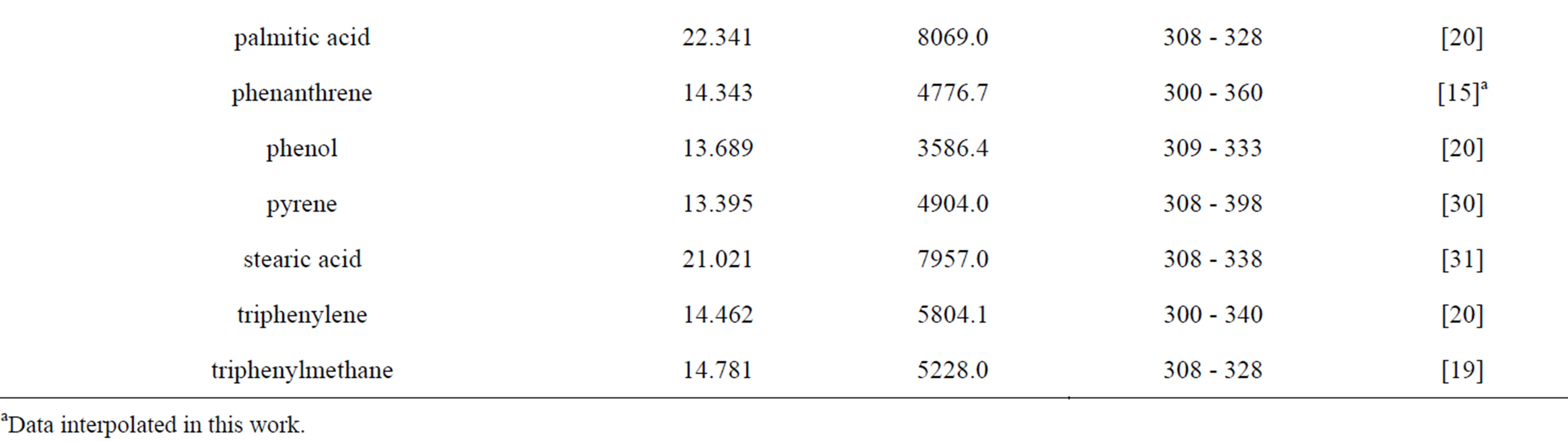
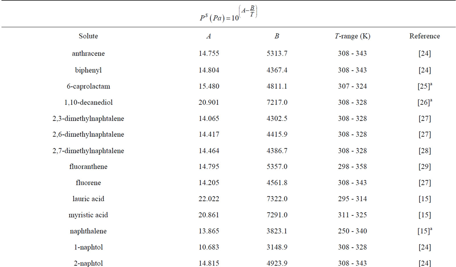
Table 6. Coefficients for sublimation pressure estimation.
aData interpolated in this work.
were split into two sets. The first set of solubility data obtained from randomly sampling 70% of the experimental data, served for the optimization of the model adjustable parameters and for training the model. The second set of solubility data was then used to test its predictive capabilities. In this step we have considered only solutes for which solubility data points are more than 20. Table 9 summarizes the key information on the two data sets, namely, the training and the test data sets together with the correlation and prediction results. This table lists the number of solubility data points used for each component and deviations in term of the AARD values obtained for both the training and the test data sets. To assess the predictive ability of the model, the two AARD values are compared. To be predictive, the model should respect the following rule: the AARD values for both data sets should be of the same order of magnitude for each component. Table 9 shows that the AARD values obtained for the test data set are in accordance with those of the training data set and are generally of the same order of magnitude. This results implies that the proposed model do not show any over-fitting problem or over prediction of the experimental solubility data. Therefore we can conclude that the predictive ability of the model is well demonstrated.
6.4.2. Ternary Systems
The study of mixed-solute systems is important because most potential applications of supercritical fluid extraction involve the removal of a desired compound from a matrix of components. However, in this section an attempt is made to predict the solubilities of mixed compounds in supercritical carbon dioxide. Experimental data provided by: Kosal and Holder [32] for mixed an
thracene and phenanthrene, Pennisi and Chimowitz [26] for mixed 1,10-decanediol and benzoic acid, Iwai el al. [33] for mixed 2,6- and 2,7-dimethylnaphtalenes are used. The solubility data of the considered compounds are very small and have an order of 10−6 - 10−3. As a consequence, we can assume that the density of the supercritical phase is that of the pure solvent, and the activity coefficient of each solute is the one at infinite dilution. In this case the only interaction parameters that are taken into account are those of solutes-CO2. Therefore predicted solubilities are estimated using Equations (6) to 13(b) and interaction parameters listed in Table 5 are directly implemented to estimate the solubility of each component in the mixture.
The interpolation results are given in Table 10, the absolute average relative deviation (AARD) obtained are generally low confirming the predictive ability of the model but have an order of magnitude considerably higher than those for the solutes in binary systems. This can be attributed to the fact that effect of solute-solute interactions is not always negligible and assuming an infinite dilution of all solutes can be inaccurate in some systems. However, there is significant experimental evidence to suggest that solute-solute interactions are important even in dilute solutions [34-36].
7. Conclusion
In this work, we have proposed the correlation and prediction of the solubility of solid solutes with different functional groups in chemically diverse supercritical fluids with a methodology based on the expanded liquid theory, in which the solid-fluid equilibrium is modeled using the local composition model of UNIQUAC. For the elaboration of the model we have considered 33 systems solid-SC fluid to built-up an exhaustive solutes solubility database consisting of more than 2218 experimental solubility data in supercritical fluids taken from literature. The proposed model achieves an overall AARD of 11.85 on a whole database and on a range of 1.16 to 29.7, these results show that the calculated solubility data are in


Table 9. Prediction capabilities of the model.

Table 10. Prediction results for solutes considered in ternary systems.
good agreement with the experimental ones. Comparison between the considered literature correlations and the proposed model was justified using comparative criteria. The model’s performance is similar and sometimes superior to the literature models considered. The advantages of this model include the following: it does not require the knowledge of critical properties of the solutes and does take into account the binary interaction between solid solute and solvent. Moreover the predictive capabilities of the proposed model were well demonstrated both for solid-solvent and mixed solids-solvent systems.
NOTES