Integration of the Classical Action for the Quartic Oscillator in 1 + 1 Dimensions ()
1. Introduction
The action
 (1.1)
(1.1)
where  equals the Lagrangian for the quartic oscillator in 1 + 1 dimensions, is integrated along an extremal and expressed in terms of the spacetime end-point data
 .
.
We begin in a well-known way by adding and subtracting the kinetic energy to the Lagrangian. Thus we obtain from (1.1), after changing the variable of integration in the remaining integral, the following equivalent expression.
 (1.2)
(1.2)
where  is the energy on the extremal (See e.g. Goldstein [1]). Equation (1.2) is the form of the action that we will start from and then derive by integrating the first term in (1.2), which we call the momentum integral, thus the desired expression for
  is obtained. (Some authors call this momentum integral the action.) For our convenience, we refer to the second term in (1.2) as the energy term. The derived action
  depends only on the end-point data in space-time.
In Part 2 Alternative derivation of the Quartic Oscillator Solution, we present an approach in which we arrive at the linearization map in [2]. This maps the solutions to Newton’s equations of motion for the quartic oscillator 1 − 1 onto those of the harmonic oscillator in a way which lends itself to integrating the momentum integral in (1.2). It involves a parametization of time t in terms of an angular coordinate  (a cyclic coordinate which takes advantage of the periodic motion of the quartic oscillator and is intrinsic to the harmonic oscillator ho). This results in the time being given by a quadrature involving a known function of
 , as in [2]. As stated in [2] R. C. Santos, J. Santos and J. A. S. Lima [3], first demonstrated the possibility of linearization of the quartic oscillator to the harmonic oscillator.
In Part 3 Integration of the momentum integral, the results in Part 2 lead to an integration of (1.2). This is a new result and an extension of the results in [3].
In Part 4 Derivation of , using the results in Part 2 and Part 3, we derive a classical action
  evaluated on an extremal in terms of space-time endpoint data and show that Hamilton’s equations are satisfied.
In Part 5 Equivalent Actions, we present two equivalent actions as variations on the result in Part 4. By equivalent we mean they are equal in value on extremals and they produce the same Hamilton’s equations.
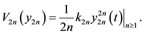
In Part 6 Conclusion, we indicate briefly how the approach in Parts 3 and 4 can be directly extended to all members of a hierarchy with potential energies
2. Alternative Derivation of the Quartic Oscillator Solution
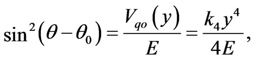
To begin with, we must establish the sign conventions implied by (1.2) for the quartic oscillator
 (2.1)
(2.1)
where 
Taking advantage of the periodicity of any extremal for the quartic oscillator qo, we execute a change of variable to the angular variable  by setting
 (2.2)
(2.2)
where

and

and E = energy on the extremal. We have opted not to change the symbol for a function when it depends on a variable through a nested function in order to avoid unnecessarily heavy notation. Making the signs explicit, (2.1)-(2.2) yield
 (2.3)
(2.3)
and
 (2.4)
(2.4)
Note, for future use (2.3) implies
 (2.5)
(2.5)
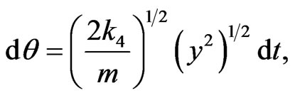
Now, we are in position to present an alternative derivation of the solution to Newton’s equations of motion (2.7) below for the quartic oscillator. It involves a parametization of time in terms of the angular coordinate. As we shall see, this results in the time being given by a quadrature involving a known function of . Now differentiating (2.4) yields
 (2.6)
(2.6)
Or from Newton’s equation of motion for the quartic oscillator
 (2.7)
(2.7)
we obtain
 (2.8)
(2.8)
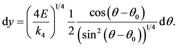
Thus, it follows from (2.3) that we obtain the equation that yields  involving
 (2.9a)
Or, it s integrated form which yields  (in quadrature) involving a known function of
 (2.9b)
The inverse of (2.9a) is given by
 (2.10a)
and it’s integrated form is given by
 (2.10b)
where the integration is along an extremal.
The equivalence to the linearization map given in [2] is specified by setting , where
  constant of the harmonic oscillator
  and
and  equals the time of the
  corresponding to
  of the
 .
.
Then (2.9b) and (2.10b) are equivalent to one half of the linearization map in [2]. The other half of the linearization map is given by
 (2.11)
Equation (2.2) plus equation (2.4) imply
 (2.12)
where  is given by (2.10b).
Finally, in this paragraph, given the end-point data how does one determine all other quantities.
One is given  and
and  on an
on an  extremal. The linearization map yields
  and
and  on the corresponding
  extremal as well as
 . This implies from (2.12) the
  time differences
 and
and , where refers to
  times, are known. Now we can set
 .
.
From [4], as a result of mapping extremals for the 
 onto extremals to the
 , we have from [4],
 (2.13)
and
 (2.14)
Now (2.13) and (2.14) imply e.g.

where  and
and  yields
 .
.
Everything else follows from the development in Part 3.
3. Integration of 
The problem of integrating (1.2) is the problem of integrating (2.1). Therefore, using (2.2) , (2.4) ,and (2.5), we obtain
 (3.1)
(3.1)
Effecting the integration by parts, where  and
and  yields
 (3.2)
(3.2)
Finally, from (2.9b), we have
 (3.3)
(3.3)
where  is given by (2.10b).
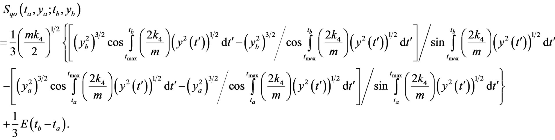
4. Determination of a 
The developments in Part 2 and Part 3 lead directly to the following determination of .
.
It follows from (3.3) that (1.2) is given by
 (4.1)
(4.1)
Therefore, using (2.10b), we obtain
 (4.2)
(4.2)
This is expressed in the endpoint variables as required. This implies
 (4.3)
(4.3)

After using (2.11) this checks with  times (2.4) for
  and
and  obviously checks.
The  -differentiations parallel the
  -differentiations and yield

 (4.4)
(4.4)
5. Equivalent Actions
Here, we present two examples of equivalent actions as variations on this result. By equivalent we mean they are equal in value on extremals and they both produce the same Hamilton equations.
First Variation:
This variation follows from the indentities
 (5.1)
(5.1)
which implies that (4.2) transforms to the expression
 (5.2)
(5.2)
Second Variation:
Equation (5.2) is equivalent to
 (5.3)
(5.3)
Comment: The signs and the limits of integration have to be carefully watched in these calculations.
The identity
 (5.4)
(5.4)
follows from 
Similarly for the  endpoint, thus we obtain the result reported in [4].
The results given in [4] were obtained before the integration result reported here in Part IV was obtained.
6. Conclusions
One can parallel the development in Parts 3 and 4 for an hierarchy with potential energies
 (6.1)
(6.1)
Starting with setting
 (6.2)
(6.2)
one can parallel Part 3.
Then integration by parts in these cases is effected by

and .
.
This then parallels the development in Part 4.
The linearization map for these cases is given in [2].