An Investigation of the Effect of the Swamping Phenomenon on Several Block Procedures for Multiple Outliers in Univariate Samples ()
1. Introduction
An outlier, or more descriptively an “outright liar” [1], is an observation (even a subset of observations) which appears to be out of line, that is, not consistent with the remainder of a data set. Such mavericks, often either innocently missed in the blind transition between data collection and computer or not so innocently slipped under the rug of “what isn’t seen can’t hurt”, should fire the curiosity and concern of researchers.
1.1. The Origin of Outliers
In most instances, the origin of outliers can be traced to one of three sources: 1) errors of measurement, 2) faults in execution, or 3) intrinsic variability. Values linked to either of the first two categories are straightforwardly rejected or replaced. Although the lack of any identifiable deterministic source does not positively rule out such causes, it should raise the possibility that intrinsic variability is the culprit. As such, the outlier must be studied “relative to some initial model for the data generation” [2: p. 247]. The recognition of an outlier is undeniably a subjective process, but one which does to some extent incorporate the crude notion of an “underlying distribution”; otherwise, how did the observation(s) “catch the eye” of the researcher and become identified as “not consistent with the rest of the sample”?
1.2. Methods for Outlier Detection
There are seven generally accepted “forms” of statistical tests of discordancy [see, 3]:
1) Excess/spread statistics are ratios of the differences between an outlier and its nearest neighbor to the range or spread of the sample [e.g., 4,5].
2) Range/spread statistics replace the numerator of the excess/spread statistic with the sample range and contrast it with another measure of dispersion, often the sample standard deviation [e.g., see 6,7].
3) Deviation/spread statistics use in the numerator a measure of distance between an outlier and some measure of central location in the sample [e.g., 8].
4) Sum of squares statistics are tests expressed as rati os of sums of squares for the reduced and total samples. Reduced sample sum of squares simply refers to the calculation based upon the total sample minus outliers [see 8].
5) Higher-order moment statistics are tests not specifically designed for assessing outliers, such as skewness and kurtosis, but which nevertheless are quite useful in this context [e.g., 9,10].
6) Extreme-location statistics take the form of ratios of extreme values (outliers to measures of central location), usually the sample mean [11-14].
7) W-statistics for normal data are simply the ratio of the square of a linear combination of the ordered sample values to the sum of squares of the individual deviations about the mean [15-17].
1.3. Treatment of Outliers
Having established the discordancy of the observation (or observations), how does one deal with the situation? According to Barnett [2: p. 247], four distinctive means of handling discordant outliers can be identified:
1) With accommodation the researcher is determined to draw inferences, typically concerning location or dispersion, regardless of the existence of outliers in the sample. Accommodation, then, concerns itself with employing robust methods, i.e., methods that protect against the existence of outliers.
2) A discordant outlier may lead to a reevaluation of the initial assumption as to the nature of the underlying probability model. As a result, the incorporation of the outlier may lead to the adoption of a new model.
3) The existence of outliers may foster the identification of important characteristics of the population. Often this can be accounted for by the development of a new “mixture” alternative probability model which assumes most of the data are coming from distribution A whereas a small probability of observations are being selected from a distinctly different population with distribution B.
4) Although widely believed to be the sole option for discordant outliers, rejection is essentially reserved for cases in which the initial probability model is considered sacred. Under this restriction, the only alternative is to dispose of the “contaminant” and proceed with the treatment of the residual sample.
1.4. Subjective Nature of Outlier Detection
The process just described is fraught with subjectivity. Fisher [18] points out the subjective nature of the researcher’s initial response as to how many, if any, outliers exist, the selection of an appropriate probability model for the data, the actual selection of an objective statistical outlier procedure, the decision as to how parameter estimates should be calculated for the test statistic (with or without the outlier present), and how the discordant outlier should be treated. She also demonstrates that the testing results can be greatly influenced by the subjective decisions adopted. Fisher then concludes:
Until a satisfactory definition of an outlier is formulated, the… researcher needing an outlier test would be well-advised to do some research on the test itself, and on the consequences of the subjective decisions required in its very execution (p. 36).
Although one purpose of this paper is to review the general outlier problem, another more substantial goal is to acquaint the reader with current work directly related to some of the problems associated with the application of outlier methods.
1.5. The Multiple Outlier Problem: Consecutive Versus Block Testing
The simplest situation to imagine is a single upper or lower, potentially discordant, outlier. Suppose, however, that the researcher observes or anticipates a cluster (k ³ 2, where k is the number of outliers) of outliers in an extreme upper and/or lower position relative to the remander of the sample. Two contrasting approaches have been proposed in the literature for dealing with such multiple outlier problems.
Consecutive testing requires that a given single-outlier procedure be applied repeatedly to outliers, one at a time, beginning with the most extreme observation and proceeding “in order of decreasing degree of deviancy, until an observation “fails” the discordancy test (i.e., moving inward) and is declared to be consistent with the rest of the data set” [19: pp. 9-10]. Alternatively, a single-outlier procedure can be applied consecutively in an outward direction until significance is reached [(e.g., 20,21]. This latter approach has an advantage that will be addressed below.
Block procedures, on the other hand, require the researcher to scrutinize suspected discordant observations as a unit. Tests have been devised for a single upperand-lower outlier pair, blocks (k ³ 2) of upper or lower outliers, or clusters (k ³ 2) of both upper and lower suspected values. Block testing is an all-or-none proposition in that all observations in the unit are declared discordant, or none of them are.
As might be expected, both approaches have inherent weaknesses. The use of block procedures requires a decision as to the number of observations one suspects to be discordant. Fisher [19: pp. 10-11] gives an excellent example that demonstrates the possible difficulties associated with this seemingly straightforward task. Consider the following three sets of data:
A: 1, 2, 3, 4, 5, 6, 7, 30, 35 B: 1, 2, 3, 4, 5, 6, 12, 20, 30 C: 1, 2, 15, 18, 19, 20, 21, 33, 35 In sample A, most observers would agree that the two upper values, 30 and 35, are suspicious. Where to draw the line to delineate the upper outliers becomes more of a challenge in sample B. And in sample C it is not even clear as to which end of the data set might, in fact, contain outliers.
Obviously, prespecification of the number of outliers is not an issue in consecutive testing. However, one problem facing the use of consecutive procedures is the effect of masking.
1.6. Masking
Barnett and Lewis define masking as “the tendency for the presence of extreme observations not declared as outliers to mask the discordancy of more extreme observations under investigation as outliers” [22: p. 114]. Take, for example, data set A above. If one wished to check for the discordancy of the values at the upper end of the sample using the consecutive testing approach, the first objective would be to apply the chosen single-outlier procedure to the observation X(9) = 35. (In this paper, X(i) refers to the ith ordered value in a given sample of elements.) If X(9) were to be declared discordant, the next move would be to test X(8) = 30 and so on until an observation failed to lead to a rejection. Presumably, X(9) and X(8) would be declared an outlier set. Masking can influence the outcome of this process, however, if the extreme nature of the observation X(8) (either a valid member of the sampled population or a discordant outlier itself) prevents the detection of X(9) as an outlier. Therefore, the masking phenomenon can halt the initiation of any consecutive testing procedure. However, consecutive application of single-outlier tests in an outward direction may avoid this problem [20,21].
Research conducted by Fisher [19] into the masking issue yielded some interesting and useful results. She used a computer simulation to generate various size samples (n = 10, 30, and 50) of pseudo-random numbers from a normal distribution. Then, according to specified criteria, a pair of outliers was located at the upper end of each ordered sample for each of the four single-outlier tests under investigation. Once all outliers were in place, a metric-free masking index was calculated by sample and averaged over sample size and test statistic. From this information a ranking of the relative susceptibility to masking of each of the four methods was created.
1.7. Swamping
Drawing again on Sample A (previously discussed in connection with masking), a simple example will demonstrate block testing’s analogue to masking: the swamping phenomenon. Suppose that, for whatever reason, a researcher wishes to apply a block procedure for outlier detection to sample A and specifies the number of suspicious observations (k) to be the upper 3. That is, the values X(9) = 35, X(8) = 30, and X(7) = 7 are to be tested as being inconsistent with the remainder of the sample against some prespecified underlying probability distribution. A block test applied to these three upper values may well declare them discordant as a unit; the extreme observations 30 and 35 have “carried” the otherwise unexceptional value 7.
The above example cites a situation with an obvious upper outlier pair; however, the use of a block test for k = 3 upper outliers may declare 35, 30, and 7 discordant. The nearest neighbor to 30 and 35, i.e., 7, may be a valid member of the population being sampled. The phenomenon may easily be simplified to a single outlier swamping a single neighbor or generalized to a situation where a cluster of k outliers swamps the nearest (n - k)th neighbor(s).
Swamping poses a potential problem for the use of any block procedure. Although the possible threat of the swamping effect has been defined and documented, very little if anything is known of the relative vulnerability of various block tests to it.
2. Methods
The approach taken to study swamping in this study was similar to Fisher’s in that it involved a simulation in which various sizes (n = 10, 30 and 50) of computer generated pseudo-random samples from a normal distribution (m = 0, s = 1) based upon a self-programmed fourparameter algorithm. Minitab (release 16.2.3) was used to generate assessments of the swamping phenomenon as well as all graphics. Outliers were placed at the upper end of each ordered sample according to specified criteria for each of the block tests being studied. Having all outliers placed, a unit-free swamping index was calculated for Special Case I (k = 1 outlier swamping its nearest neighbor), Special Case II (k = 2 outliers swamping a third value) and Special Case III (k = 3 outliers swamping a fourth value, and the simplest example of the most generalized case of k outliers swamping the nearest (n − k)th neighbor).
2.1. Example: Special Case I
Given a specific sample and a particular block test, for a given a-level there exists a point above the mean, at or beyond which any sample value and its next lowest “core” neighbor will be declared discordant, as a unit. Define O1 as the point at or beyond which a given block test will declare  and
and  both discordant upper outliers, i.e.,
  will swamp
 . Define d1 as
 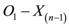 which represents the relative susceptibility of that test to swamping.
Defining d2 as  (where
  is the mean of the n − 1 “core” of observations), the ratio of d2 to d1, or
 , provides a metric-free indication of a block test’s susceptibility to the swamping phenomenon. The greater the magnitude of the swamping index, the greater the susceptibility of a given test to the swamping phenomenon (see Figure 1) (Given more than a single outlier, a centroid value (
 or median) representing the outliers is suggested for use in determining the swamping index).

Figure 1. Outlier placement and swamping index.
The block procedures evaluated in the above manner were:
 sum of squares statistic [8] where,

 excess/spread statistic [23]
 deviation/spread statistic [24]
 variation of sum of squares [25]
where , the absolute deviation of
  from the sample mean;
 are the values of the
  in ascending order,
 ;
;
 the mean of all the
  ‘s; and
  the mean of the
  lowest
  ‘s, i.e.,
 .
.
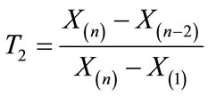
2.2. Test Selection and the Swamping Consideration
This study focused on four specific block procedures for multiple outliers. Test T2 was restricted in its usefulness due to its design (only appropriate for k = 2 outliers), as well as limitations in the availability of distributional information. It is recognized that any attempt at outlier test selection is influenced by many considerations. The researcher must contemplate the goals and objectives of the study, existing knowledge about the population distribution, as well as personal and practical issues as they relate to the application of such procedures.
3. Results
Those hoping to avoid the swamping effect when adopting the block approach would certainly wish to avoid test T3 under small sample conditions, n = 10 (see Table 1 for a summary the relative susceptibility of each test to swamping, for each case; graphical presentations of the results are provided by Figures 2-5). In fact, when samples are relatively large (n = 30 to 50) and k is relatively small (e.g., 2 or 3), or when the reverse is true, one would also be ill-advised to apply T3. An investigator in the exploratory phase primarily interested in population characteristics might wish to take a more “conservative” approach if very small samples or very few outliers are the rule. For instance, the situations outlined above might be better served by the application of test T2, if appropriate; otherwise, T1, or even T4 would be suitable middleof-the-road choices.
On the other hand, access to a larger data set with suspicion of more than 2 or 3 of these maverick observations points toward T3 as more appropriate. Within this context, test T3 exhibited less vulnerability to swamping than T1 or T4, and might be considered the most satisfactory technique. Quite clearly, test T4 stands alone as most susceptible to swamping given larger samples with a higher frequency of potential outliers.
As general as these recommendations may be, certain explicit inclinations in the behavior of these tests under tightly controlled situations do make the researcher

Table 1. Ranked susceptibility of swamping (most to least) and mean swamping index (S, in parentheses) of block outlier tests.
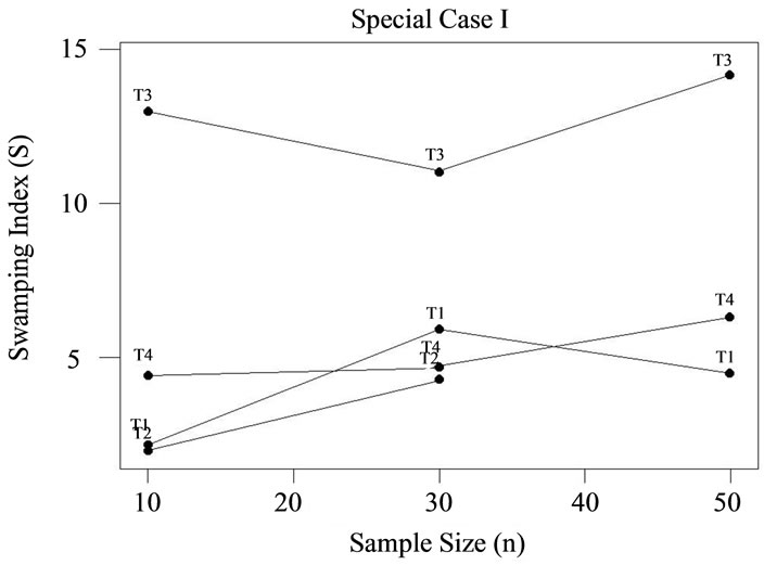
Figure 2. Swamping index by test: Special case I.
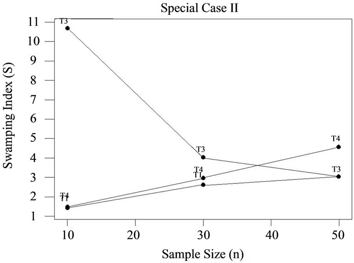
Figure 3. Swamping index by test: Special case II.

Figure 4. Swamping index by test: Special case IIIa.
aware of important considerations in the selection of any block procedure. Given the evidence that tests T1, T2, and T4 became more susceptible to swamping as sample size increased (and the number of potential outliers remained constant), one should weigh carefully the decision to adopt a block technique as opposed to a consecutive one,

Figure 5. Swamping index by test: Special case IIIb.
since Fisher [19] has demonstrated that the influence of masking is inversely related to n, for this latter approach. However, it was precisely this characteristic, the susceptibility to swamping being inversely related to sample size, which made test T3 more attractive as sample size and k increased.
Although an exception existed (n = 50, T4), this study revealed that for a given test and sample size, vulnerability to the swamping effect decreased as the block of potentially discordant observations grew. Therefore, regardless of the procedure being considered by the investigator, as the number of rogue observations mounts the likelihood of interference by swamping appears to diminish, and therefore test selection based upon this criterion becomes less productive.
In summary, if one standard in test selection is swamping, tests T1 and T2 would be recommended as most efficacious for small samples in general (especially if normality is assured), as well as for large samples with relatively small blocks of outliers. Conversely, T3 becomes most desirable under circumstances where a sizable block of outliers appears to exist in a relatively large sample, but T4 should be avoided.
4. Discussion
It is noteworthy that Fisher [19] found an unusual quality in one of the tests she evaluated. Upon placing the pair of outliers in her samples, she found a tendency for one test to place the second outlier inside the first. This occurred 81% of the time for samples of size 30 and 94% of the time for samples of size 50. It should also be noted that this same test was least susceptible to masking and in terms of outlier definition (another aspect of Fisher’s study was to investigate the definitions of “outlier” inherent in the several single-outlier tests under evaluation), and it was the least conservative. She concluded that this test “defined as outliers observations which were relatively closer to the [“center” of the sample] than the other tests did” (p. 49).
Findings in the swamping study indicated a similar phenomenon with the single outlier (or “centroid” of 2 or 3 outliers in cases II and III, respectively) being placed within the upper boundary set by  more often with increasing sample size for T1 and T4, and yet T2 and T3 were inversely related to n in this respect. This could simply indicate, as suggested by Fisher’s [19] results, that those block tests exhibiting this enigma rather frequently are quite liberal in terms of outlier definition. However, this peculiarity deserves further thought, discussion, and investigation.
The need to assess and rank singleand multiple-outlier tests in terms of their relative degree of “conservatism” concerning outlier definition, as well as “susceptibility” to such phenomena as masking and swamping may assist with developing the generalized outlier methodology alluded to by Barnett and Lewis [3], Rosner [26], and others.