Mathematical Model of Leptospirosis: Linearized Solutions and Stability Analysis ()
1. Introduction
In Thailand, leptospirosis occurs mainly in the rainy season, with an increase in cases beginning in August, reaching a peak in October, and beginning to fall in November [1]. Leptospirosis in contaminated material may infect a person or other mammal. The bacteria penetrates the blood vessels, multiplies and infects several organs. Acute disease may be observed in several species, especially humans and dogs. In livestock sub-acute or even endemic, leptospirosis is generally observed. Infection induces antibody production in the animal renal carriers, shedding leptospirosis in their urine several weeks or even months after infection [2]. In humans, symptoms are generally flu-like, but the disease can result in liver damage and renal failure.
In this study, a compartmental model, with human susceptible-infective-removed-susceptible (sirs) model and vector susceptible-infective (si) model, [3-5] was used to examine the dynamical behaviour of the spread of leptospirosis, a vector borne disease. The sir model has been used to describe the transmission dynamics of many diseases. J Holt et al. 2006 [6] used this model to understand the behavior of infection in an African rodent of Tanzania. In Thailand, W. Triampo 2007 [1] introduced a deterministic sir model for the transmission of the spread of leptospirosis for the Thai population. In this work a modification of the sir model, which is used to describe the general transmission dynamics of leptospirosis, is proposed, and thresholds for changes in stability are found.
2. Model
The sir model has both human and vector populations. The vector in this case are rats. The human population is divided into three subgroups; susceptible humans , infected humans
 , and recovered humans
 . The vector population is divided into two subgroups, susceptible vectors
  and infected vectors
  [1].
[1].
The following assumptions are considered in the model, as in Triampo [1], reproduced below:
• Newborns are not immunized and are therefore vulnerable instantly;
• All compartments of vector and human populations are well-mixed and therefore are spatially uniform;
• Humans can be infected by infected vectors but not by infected humans;
• Infected humans cannot infect susceptible vectors;
• Susceptible vectors  become infected vectors
  instantly, with no incubation period needed for the infectious agents (leptospira) to develop.
In addition, we assume that:
• Perfect maternal transmission occurs, that is, new borns are susceptible if they are born to a susceptible mother and infective if they are born to an infective mother;
• Disease transmission is dependent on the product of the density of susceptibles and the infected (instead of the frequency of transmission: this difference disappears after normalisation);
• The total population remains constant.
Figure 1 shows the dynamics of the transmission of leptospirosis based on the assumptions above.
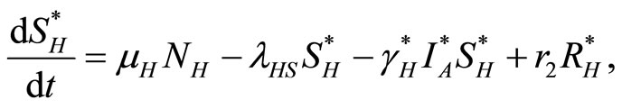
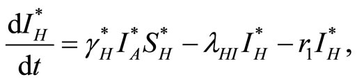
The law of mass action, where rates are proportional to the size (number) of each component, leads to the following set of coupled ordinary differential equations:
 (1)
(1)
 (2)
(2)
 (3)
(3)
 (4)
(4)
 (5)
(5)
where * indicates a non-normalised variable.
The variables in (1)-(5) are normalised, giving proportions in each compartment, based on the assumption that the population remains constant, by letting
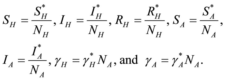
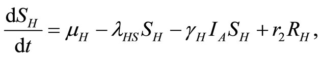
Then Equations (1)-(5) become
 (6)
(6)
 (7)
(7)
 (8)
(8)
 (9)
(9)
 (10)
(10)
By using the constraints  and
and  the above system of equations can be simplified to:
 (11)
(11)
 (12)
(12)
 (13)
(13)
Here we have omitted the equations involving ,
, and used the constraints to make the system into only three compartments.
3. Equilibrium Points
Equilibrium points are found by setting the right hand sides of (11)-(13) equal to zero. This gives two equilibrium points in the feasible region. The disease-free equilibrium point  and the endemic equilibrium point
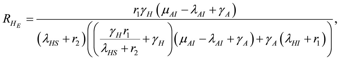
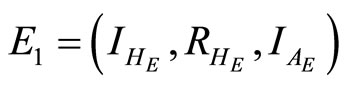 . After rearrangements this gives the endemic equlibrium point
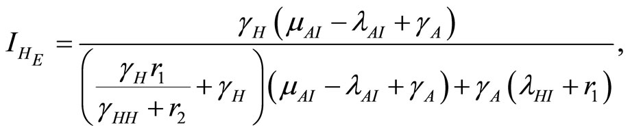 (14)
(14)
and
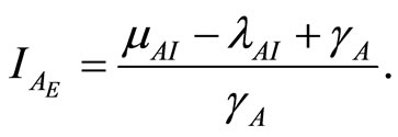 (16)
(16)
When  then
then  and
and . In this work the spreading of infection between human and vector is assumed to depend on rainfall. This means that the basic reproduction number
  depends on
 . Equations (14)-(16) can be simplified to:
 (15)
(15)
 (17)
(17)
 (18)
(18)
 (19)
(19)
where  and
and 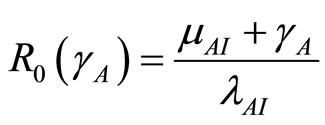 which is the basic reproduction number [1]. Infection in humans is described by an SIR model, but as animals do not recover, the disease in this vector is described by a SI process.
4. Local Stability Analysis
In this section the local stability analysis of (11)-(13) at steady-state is carried out. The Jacobian matrix of the system is given below:
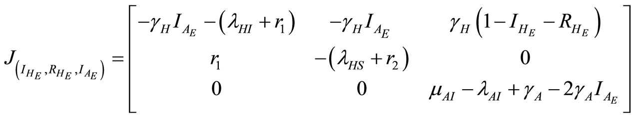 (20)
(20)
The eigenvalues at  are
are
 (21)
(21)
The eigenvalues of the Jacobian matrix in (19) of the disease-free steady state have negative roots which are independent of any parameter. These eigenvalues tell us that there is only one case of solution, i.e., all eigenvalues are real and equal. The negative root condition is found by considering the eigenvalues (20). Now 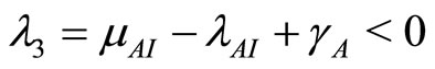 when
when  so
so
 . So the system is stable at the disease-free state since
 .
.
In the case of the endemic disease state, the eigenvalues at  are
are
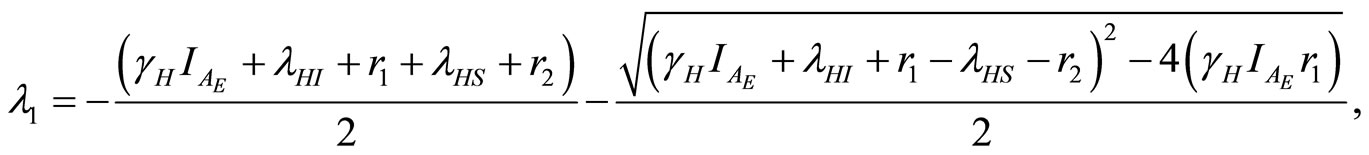 (22)
(22)
 (23)
(23)
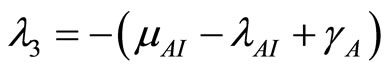 (24)
(24)
The following three theorems follow immediately from [7]:
Theorem 1 The disease-free state at  is locally asymptotically stable if
  and unstable if
 .
.
Theorem 2 The endemic state at  is locally asymptotically stable if
  and unstable if
 .
.
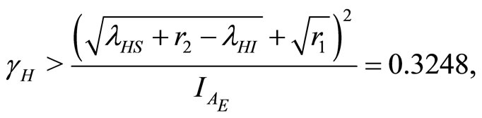
From theorem 2 and theorem 2  is a bifurcation point of the system where
 . The expression above shows the relationships between
  and
and  including bifurcations at
  and
and  respectively. The parameters utilized in this calculation are


 and
and . Letting
  and
and  and using the above theorems the bifurcation point
  occurs when
  as displayed in Figures 2(a)-(c) In the proof of the following theorem, the Liapunov function is used to show that the disease free state at
  is globally asymptotically stable.
Theorem 3 If , the existence of local stability implies its global stability [4].
Proof. Define the Liapunov function as .
.
Then

 (25)
(25)
This concludes the proof.
Then from theorem 2 the disease-free state at  using
using  is globally asymptotically stable since
  as shown in Figure 3.
5. Numerical Solutions
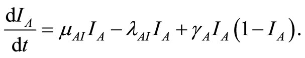
Numerical calculations were utilized for solving (11) and (12), however, an analytical solution was found for (13). The solutions were used to analyze and examine the behavior of the model and determine whether the results converged.
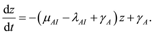
From (13)
 (26)
(26)
Divide both sides by , then let
  and
and . Then
 (27)
(27)
Multiply both sides by  to get
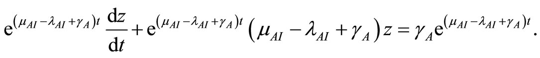
This simplifies to


 (28)
(28)
where  is a constant determined by the value of
  at
at .
.
Let
 (29)
(29)
Here (29) is the analytical solution of (13).
The negative root condition is found by examining (24) and (29).
As the eigenvalues  and
and  from (22) and (23) must be real, the following inequality is required:
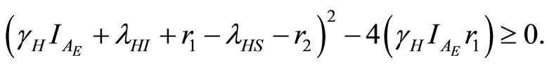 (30)
(30)
Then from (30)
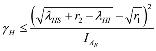 (31)
(31)
and
 (32)
(32)
when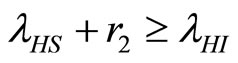 . The cases are divided as will follow. The results correspond when using


 .
.
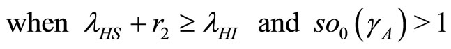
5.1. Case 1
All eigenvalues are real and distinct at the steady state . When
  since
since  , then the steady-state solution at
  is stable.
Figure 4(a) shows the stable steady state using a phase portrait. The graph of the numerical solution converges to the equilibrium point . The parameters

Figure 1. Flowchart of the transmission dynamics of leptospirosis.
used are  and so
 . Figure 5(a) shows the solutions of
  and
and  over time. The values of
  and
and  are limited by
 .
.
At 
 (33)
(33)
 (34)
(34)
 (35)
(35)
When  then
then  so the equilibrium point
  is stable.
Figure 4(b) is the phase portrait of the solution. The graph of the numerical solution converges to an equilibrium point . The parameters are
  and so
  . So
. So  is stable. Figure 5(b) shows the solutions of
  and
and  over time. The values for
  and
and  are limited by
  . In the following cases, these is no
  because the values of (20) can not be found.
5.2. Case 2
All eigenvalues  and
and  from (21), (22) and (23) are real. Two eigenvalues are equal while the third is distinct.
Now
 (36)
(36)
 (37)
(37)

Figure 3. Graph shows global asymptotic stablity at .
.
 (38)
(38)
Figure 6 shows the phase portrait for this case. The graph of the numerical solution converges to the equilibrium point . The parameters used are
  and so
 so
so  is stable. Figure 7 shows the solutions of
  and
and  over time. The values of
  and
and  are limited by
  .
.
5.3. Case 3
Two eigenvalues are complex while the third is real.
 (39)
(39)
 (40)
(40)
Figure 6 is the phase portrait of the solutions. The graph of the numerical solution converges to the equilibrium point  where the parameters are
  and so
  so
so  is stable. Figure 7 shows the solutions of
  and
and  over time. The values of
  and
and  approach the value of
  .
.
6. Discussion and Conclusion
The important factors of the spreading of leptospirosis are the rate of transmission of leptospirosis from an infected vector to a susceptible human  and the rate of transmission of leptospirosis from an infected vector to a susceptible vector
  [1]. These two factors depend on rainfall. A summary of the two factors is included here:
1) The spreading of leptospirosis has two states: the disease-free state and the endemic state. The occurence of a state depends on . If
. If , then the disease-free state will occur but if
  then the endemic state will occur as shown in Figures 2(a)-(c).
2) For the disease-free state, a Liapunov function was used to prove that it is globally asymptotically stable. So for any initial population, over a long time, the population will converge to the disease-free steady state, as shown in Figure 3.
3) Two factors impact on the endemic state case:  and
and . Before the convergence point
 (41)
(41)
when  then
then 


 and
and  which can be classified as below:
I. For  the number of infected humans initially increases before decreasing to the endemic state while the number of recovered humans increases to the endemic state. This is shown in Figures 5(b) and 7.
II. For  the number of infected humans initially increases before decreasing to the endemic state while the number of recovered human initially increases before decreasing to the endemic state. This is shown in Figure 8.
4) The death rate of the infected vector population is equal to or greater than the natural birth rate of the infected vector population.
5) The time to convergence to the disease free state is longer than the time to convergence to the endemic state because the amount of time before the disease disappears is longer than that of the endemic state. This reflects what would happen in the real world.
7. Acknowledgements
This research is supported by The Center of Excellence in Mathematics, CHE, Thailand.
Nomenclature
 : number of humans susceptible (non-normalised).
 : number of humans infected (non-normalised).
 : number of humans recovered (non-normalised).
 : number of vectors susceptible (non-normalised).
 : number of vectors infected (non-normalised).
 : time measured in days.
 : natural birth rate of human population.
 : human population.
 : natural death rate of susceptible and recovered humans.
 : rate of transmission (non-normalised) of leptospirosis from an infected vector to a susceptible human, varying with rain fall.
 : rate immune individuals become susceptible
  again.
 : natural death rate of infected humans plus the death rate due to the infection.
 : rate infected humans can be cured by antibiotic medicines and become immune.
 : natural birth rate of susceptible vectors.
 : natural death rate of susceptible vectors.
 : constant natural birth rate of infected vectors.
 : natural death rate of infected vectors plus the death rate due to the infection.
 : rate of transmission (non-normalised) of leptospirosis from an infected vector to a susceptible vector, varying with rain fall.
 : proportion of humans susceptible (normalised).
 : proportion of humans infected (normalised).
 : proportion of humans recovered (normalised).
 : proportion of vectors susceptible (normalised).
 : vector population.
 : proportion of vectors infected (normalised).
 : rate of transmission of leptospirosis from an infected vector to a susceptible human, varying with rain fall.
 : rate of transmission of leptospirosis from an infected vector to a susceptible vector, varying with rain fall.
 : disease free equilibrium point.
 : proportion of humans infected at equilibrium point (normalised).
 : proportion of humans recovered at equilibrium point (normalised).
 : proportion of vectors infected at equilibrium point (normalised).
 : endemic equilibrium point.
 : basic reproduction number.
 :
:  eigenvalues.