Mathematic Model of Green Function with Two-Dimensional Free Water Surface ()
1. Introduction
The analysis of interaction between waves and ship by singularity distribution method involves calculation for Green function [1,2]. After computer was used to compute hydrodynamics, finding a fast way to calculate Green function became a science research work [3,4]. Newman [5] published theories and numeric methods for computing the velocity potential, and its derivatives, for linearized wave motions due to a unit source with harmonic time dependence beneath a free surface. Shen [6] gave an approximated algorithm to estimate Green function and its derivatives by using truncated series expansion of the Green function were to avoid the conventional timeconsuming numerical integration. Zhu [7] showed a subdomain approximate method to evaluate frequency domain free surface Green function with sufficient accuracy. Yang [8] compared the classical Green function and a simpler Green function associated with the linearized free-surface boundary condition for diffraction radiation by a ship advancing through regular waves. Shen [9] proposed the ordinary differential equations about depth Green function and its derivative, and a rapid Green function calculation method combining solving ordinary differential and interpolation between nodes. John [10,11] showed a variety of representations for Green function with finite and infinite water depth. Other expressions for the free-surface Green’s function, in two dimensions and for infinite water depth, have been improved by Liu [12], Thorne [13], Kim [14], Greenberg [15], Macaskill [16], and Dautray and Lions [17]. Some representations for the Green’s function are also discussed in [18-21]. A more general two-dimensional water-wave problem that considers surface tension is treated in [22-24].
This paper will discuss mathematic model of Green function with two dimension free water surface. In Section 1, the Green function is represented by using two parameters. In Section 2, intrinsic properties of Green function are discussed. In Section 3, special value of Green function is given for vertical line and horizontal line. In Section 4, the derivation of Green function is obtained for two dimension free water surface.
2. Two Dimension Green Function
Suppose velocity potential φ satisfies Laplace equation:
 (2.1)
(2.1)
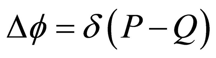
Here P is field point ,
, . Q is source point
 ,
, . The right of equation is delta function. The boundary condition is:
 (2.2)
(2.2)
Here F is complex potential. On the free surface y = 0, velocity potential satisfies linear condition. We easy find its solution [12]:
 (2.3)
(2.3)
Here  is called green function, I is principle value integration of below

where the integral lower limit is 0, The integral upper limit is ¥,  is zero point of denominator, upper subscribe (¥, K) shows that it is principle value integration at point
 . From the expression of integration, the value I is determined by the parameters of K,
  ,
, . Let unit transfer as
 (2.4)
(2.4)
The principle value integration may be written as
 (2.5)
(2.5)
where  is called H-function with two parameters:
 (2.6)
(2.6)
here parameters take value as .
.
3. Intrinsic Properties
First, confirm that you have the correct template for your paper size. This template has been tailored for output on the custom paper size (21 cm × 28.5 cm).
Let Re(H) and Im(H) are real part and imaginary part of  respectively. We will discuss Re(H) and Im(H) with parameters a and d.
3.1. Parameter ( = 0
In the case d = 0, from expression of , we easy know, Im(H) = 0, and
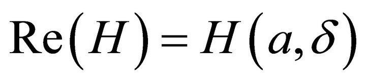 , or
, or
 (3.1)
(3.1)
Above formula is principle value integration with one parameter, and may be rewritten as:

We easy obtain

And by adopting subsection integration method, we have:
 (3.2)
(3.2)
So that:

Here constant is:
 (3.3)
(3.3)
At last, we have
 (3.4)
(3.4)
The integral value of H(a,0) is shown in Figure 1. From Figure 1, we have below theorem:
Theorem 1. 1)  as
as .
.
2) 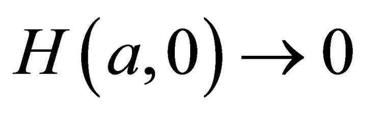 as
as .
.
3) The lowest value 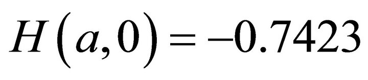 when a = 1.347.
4) On the domain , the curve is down.
5) On the domain , the curve is rise.
3.2. Parameter ( ( 0
If the value of parameters d is not zero, we have
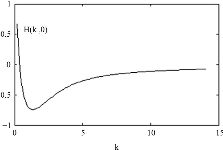
Figure 1. One parameter principle value integration H(a, 0).

And:
 (3.4)
(3.4)
From above formula, we have below theorem:
Theorem 2. The real part of function  is Symmetric function, or
 . The imaginary part of
  is antisymmetric function, or
 ;
;
By using expression of Green function, we have ordinary equation:

So that we may express Green function as:

Using series expansion, we get:
 (3.5)
(3.5)
Here constant Ca = −0.577215. It is easy to calculate H-function by using above formula with given parameters. The numeric results are shown in Figures 2 and 3.

Figure 2. Real part Re(H) varied with parameters.

Figure 3. Imaginary part Im(H) varied with parameters.
3.3. Property of ( = (/2
Considerd = p/2, then H-function may be written as:
 (3.7)
(3.7)
Here

4. Properties of Green Function
By using expression of H-function, we have below theorem:
Theorem 3. Consider field point  and source point
  are below free surface, the Green function may be expressed as:
 (4.1)
(4.1)
Here
 (4.2)
(4.2)
where constant Ca = –0.577215.
4.1. Vertical Line
Consider field point  and source point ζ = ξ + iη take value at vertical line
 ,
, . According to the define of X, we have X = –1, or d = 0. In this case, the Green function is
 (4.3)
(4.3)
From above formula, last term is imaginary part of Green function, others at right is real part. Above formula also show that the Green function may represented by using H-function at d = 0.
4.2. Horizontal Line
Consider field point  and source point ζ = ξ + iη take value at horizontal line S:
 ,
, . According to the define of X, we have
  . In this case, the Green function is
 (4.4)
(4.4)
Here

On the free surface, y0 = 0, X = ±i. Consider X = –i, or δ = π/2, the Green function can be written as:
 (4.5)
(4.5)
On the free surface, the Green function may represented by using H-function at .
.
5. Derivation of Green Function
We know, the derivation of potential are:
 (5.1)
(5.1)
It is easy to obtain the derivation of Green function as:
 (5.2)
(5.2)
Consider field point  and source point ζ = ξ + iη take value at vertical line S:
 ,
,  , we have formula of two parameter
 :
:

6. Conclusion
In the paper, the Green function is simplified from integral formula by using two parameters. The intrinsic properties of Green function are discussed on vertical line and horizontal line. The derivation of Green function is obtained by using complex theory.
NOTES
#Corresponding author.