Electrostatic Attraction and Repulsion Explained and Modelled Mathematically Using Classical Physics
—A Detailed Mechanism Based on Particle Wave Functions

Declan Traill

Melbourne, Australia.

DOI: 10.4236/jamp.2024.124065                

Abstract

The phenomenon of electrical attraction and repulsion between charged particles is well known, and described mathematically by Coulomb’s Law, yet until now there has been no explanation for why this occurs. There has been no mechanistic explanation that reveals what causes the charged particles to accelerate, either towards or away from each other. This paper gives a detailed explanation of the phenomena of electrical attraction and repulsion based on my previous work that determined the exact wave-function solutions for both the Electron and the Positron. It is revealed that the effects are caused by wave interactions between the wave functions that result in Electromagnetic reflections of parts of the particle’s wave functions, causing a change in their momenta.

Keywords

Electrostatic, Electron, Positron, Coulomb, Force, Attraction, Repulsion, Wave, Function, Electric, Magnetic, Radiation, Pressure, Shell, Theorem, 3D, Computer, Model, Quantum

1. Introduction

It is universally accepted that like charges repel and unlike charges attract and Coulomb’s Law describes this behaviour very well. However, it is seldom questioned as to why this is so. What is it about particles that make them charged and what causes the attraction or repulsion to occur? There is very little work done on examining and trying to understand what mechanisms could cause this behaviour between fundamental physics particles. The only work I can find that touches on this is that done by James Clerk Maxwell [1] in his foundational work on Electromagnetism. He attempts to explain the effects of magnetism as pressure between spinning loops of an ethereal type of fluid that fills space and supports the existence of magnetic fields. He says “…pressure in the equatorial direction arises from the centrifugal force of vortices or eddies in the medium having their axes in directions parallel to the lines of force”. In a similar sort of line of thought, I have analysed the problem given the insight I have gained from my work on determining the electron/positron wave functions, comprised of Electromagnetic waves.

In earlier work [2] [3] , it was found that the wave functions of the Electron and Positron each comprise a three-dimensional spiral wave that is rotating, such that there is a flow of wave phase either outwards or inwards as it rotates. This direction of the phase flow is what determines if the particle is negatively or positively charged. These spiral wave structures can be further broken down into the sum of inwardly and outwardly travelling spherical waves. The sum of the energies of the Electric and Magnetic fields in these waves over a small volume of space (containing the particle at the center) yields that particle’s rest mass energy equivalent [4] .

There is an energy balance between the inward and outward waves (i.e. the magnitude of the energy of the inflowing waves equals that of the outflowing waves) resulting in no net energy loss/gain for the particle as a whole. This is a guaranteed feature of the wave functions, as they are mathematical solutions to both the Classical and Schrödinger wave equations; thus, they represent temporally stable wave structures.

For an Electron there exists, at any point in space, a phase flow of the wave function’s waves outward with respect to the Electron’s centre. The phase flow causes the attraction/repulsion, classically associated with the electric field (Coulomb’s Law) when it interacts with other charged particles’ wave functions. As one moves further from the Electron’s centre, the amplitude of the waves decreases, and so too does the electric field and its associated Coulomb force due to these waves (i.e. lower wave amplitude = lower momentum in waves = lower force on other charged particles).

When the electric field of the electron interacts with other charged particles (for example, another identical electron), the inward and outward waves of each Electron overlap in space. When this happens, at the interface between the two electrons (at exactly equal distances between each electron’s centre), the two outward waves will form a standing wave and the two inward waves will form a standing wave—each of these standing waves will have no phase flow in space as an equal amount and frequency of each Electromagnetic wave is coming from each side of the interface location in space. Thus, the nodes of the standing wave at this point will not be moving.

As the overall wave function of the electron has an outward phase flow, when a stationary node forms at this midway point, the outward wave will be reflected and Doppler shifted to form an inward wave of higher frequency than usual. In the space between the two Electrons, the nodes from the electron’s centre to the midway point become progressively slower, until at the midway point, the node stops completely. Thus, the interface between two electrons provides a frequency conversion, or momentum change, to the inward/outward waves in the region between the two Electrons. These frequency/momentum changes will propagate through each node of the Electron’s wave function to the electron’s centre causing the whole electron to move—thus, the electron has been accelerated.

The aim of this paper and the modelling results it presents is to demonstrate that the known attractive or repulsive force that exists between charged particles can be accurately modelled and explained theoretically using Classical Physics when the wave structure of charged particles (such as the electron and positron) is taken into consideration.

2. Method

The interaction between the dynamic, three-dimensional, Electromagnetic wave structures of two or more such charged particles can account for the observed attraction/repulsion through an incident radiation pressure at the node interfaces in the space occupied by the particles’ wave structures.

When Electromagnetic waves reflect perfectly, they impart a radiation pressure equal to twice the incident radiation pressure. So, by identifying all the points in space where such reflection is occurring, over the region containing the two (or more) charged particle wave functions that are interacting, it is possible to calculate an overall radiation pressure that is acting on the particle. When this is done (for example, between two Electrons, two Positrons, or an Electron and a Positron) the total force acting on each particle can be determined. Then, by using Newton’s 2^nd Law (F = ma), the acceleration of each particle can be determined. For two Electrons or two Positrons, the wave reflections occur predominantly in the space between the two particles—thus, causing an outward force that repels each particle from the other. For an Electron and a Positron, the regions that reflect are predominantly outside the two-particle system—thus, causing an inward, attractive force between the two particles. The following two figures are plots of the magnitude of the x-axis component of the reflected Electromagnetic energy for two different modelled particle configurations: 1) Two Electrons, 2) An Electron and a Positron.

The amount of power coupling between the two particles (electrons) depends on the amount of reflection of the waves from each particle on the other. This amount depends on the minimum RMS power of the two interacting waves along the axis connecting the two particle centres (the x-axis in this model), as the waves can only reflect when equal but opposite Electromagnetic wave components meet at the reflection point.

The regions in the space occupied by the two wave functions that have the most reflected power differ between two particles with the same charge, Figure 1, where the reflected power is mostly in the space between the particle centers, thus causing repulsion; and between two oppositely charged particles, Figure 2, where the reflected power is mostly in the space outside of the two particles, thus causing an inward, attractive force.

Figure 1. Wave reflections between two Electrons. Wave reflection occurs predominantly in the space between particle centers.

Figure 2. Wave reflections between an Electron and a Positron. Wave reflection occurs predominantly in the space outside of the two particle centers.

The power values of each Electromagnetic wave are calculated from the Poynting Vector (vector cross product) of the RMS Electric and Magnetic field values of the minimum power of the two interacting waves at each point [5] :

${\epsilon }_{RMS}=\frac{E}{\sqrt{2}}$ (1)

Electric energy density:

$\therefore u_e=\frac{{\epsilon }_0\cdot {\epsilon }_{RMS}^2}{2}=\frac{{\epsilon }_0\cdot E^2}{4}$ (2)

Poynting vectors (power flow):

$S_1=E_{RMS1}\times H_{RMS1}$ (3)

$S_2=E_{RMS2}\times H_{RMS2}$ (4)

Minimum power of the two waves (one from each particle) at a point in space:

$S_{\min }=S_1\wedge S_2$ (5)

There is an additional factor that determines the amount of power coupling between the two particles—the relative orientations of the polarizations of the two waves and how much they align and thus, reflect off each other. As the interface area between the two electrons is a circle, the amount of coupling between the two Electromagnetic waves will vary sinusoidally (around this circle) with the angle difference between the polarizations of the two waves.

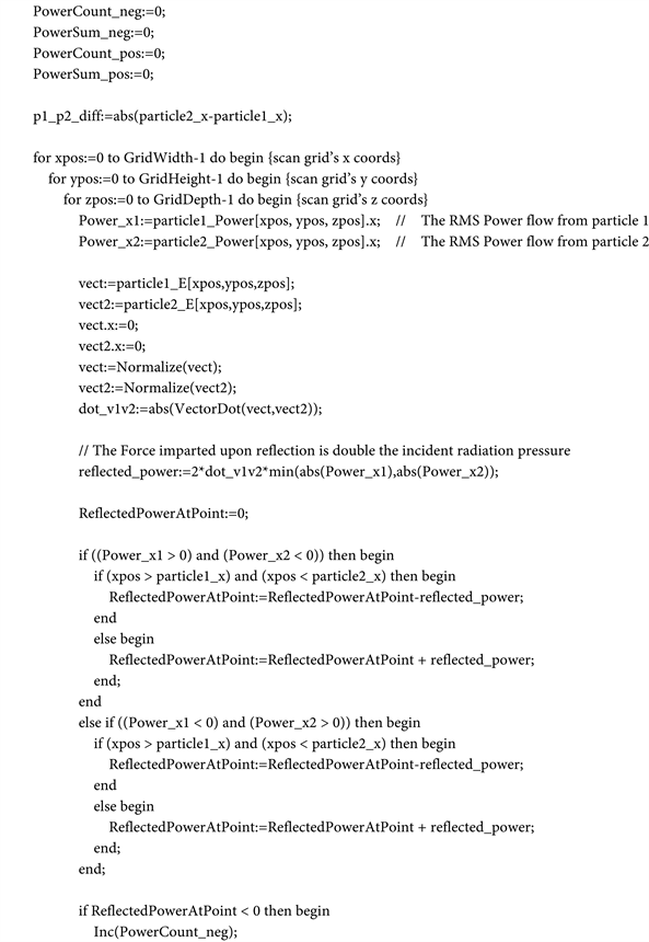
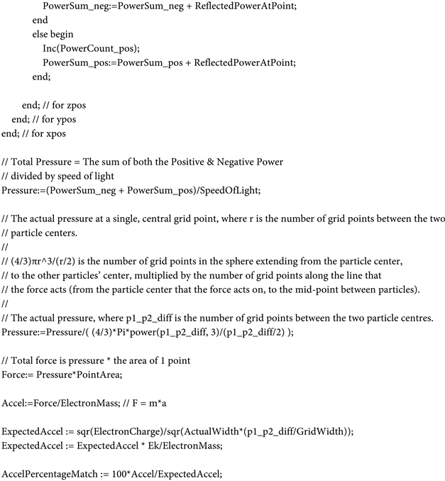
However, this effect is taken care of in the maths as the dot product of the two Electromagnetic waves is used to determine the amount of reflection during the calculation of the total reflected power between the two particles’ wave functions. See Appendix for an extract of the code used to determine the acceleration between the two electrons.

Alignment (dot product) of the two particles’ Electric fields (using Normalized E vectors):

Normalized electric field vectors: $E_{N1}$ and $E_{N2}$ :

$E_{N1}=\frac{E_1}{\left|E_1\right|}$ (6)

$E_{N2}=\frac{E_2}{\left|E_2\right|}$ (7)

$E_{Ndot}=E_{N1}\cdot E_{N2}$ (8)

$P_A$ is the RMS Electromagnetic power flow at each area element within the modelled region.

Reflected Power between two particles’ wave function at the same point in space:

$P_A=2\times E_{Ndot}\times S_{\min }$ (9)

The Power value obtained is then converted into a pressure by dividing by the speed of light [6] . To work out the actual force between the two particles, we need to simplify the calculation by conceptually reducing each particle to a point particle at its wave function centre, with an effective area of interaction of one grid point in the model. The force between them is due to wave reflections at the mid-way point between them—where waves from each side are equal.

$p_A=\frac{P_A}{c}$ (10)

In a similar way to the Shell Theorem for gravity, where the force between two bodies due to the mass of one spherical body can be treated as all coming from a single point at that spherical body’s centre of mass, the attractive/repulsive force between charged particles can be treated similarly, but centered around the charged particle’s center of charge.

If we start from the situation where both particles are together almost at the same point, then there is a single grid point of area interacting between them. As the particles move apart, the volume of the sphere from each particle’s centre to the center of the other particle’s wave function represents all of the contributing grid points to the total force attributed to the single central point.

As the volume of a sphere is:

$V=\frac{4}{3}\pi r^3$ , (11)

where r is the distance between the two particle centres (on the x-axis).

$r=\left|x_1-x_2\right|$ and $r>0$ (12)

If d is the number of grid points between the two particle centres, rather than r (which is in meters):

$d=\frac{r}{dx}=\frac{1}{dx}\left|x_1-x_2\right|$ (13)

Expressing this in terms of d:

$V=\frac{4}{3}\pi d^3=\frac{4}{3}\pi {\left(\frac{r}{dx}\right)}^3$ (14)

This quantity is a dimensionless number (a number of grid points).

At each grid point in the model, there is a pressure element $p_A$ . The actual force at each grid point can be determined by multiplying this pressure element by the area of a single grid point.

If $F_A$ is the infinitesimal Force element at each location in the 3D volume being integrated. It is equal to the infinitesimal pressure element multiplied by the infinitesimal area over which the pressure acts:

$F_A=p_A\cdot dA$ (15)

In the model, to calculate the Force between the two particles, first a sum of the finite model force elements is calculated:

$F_{sum}={\displaystyle {\sum }_{x=0}^{x=x_{\max }}{\displaystyle {\sum }_{y=0}^{y=y_{\max }}{\displaystyle {\sum }_{z=0}^{z=z_{\max }}\left(F_A\right)\text{d}x\cdot \text{d}y\cdot \text{d}z}}}$ (16)

Then, this sum needs to be divided by the number of grid points within the sphere from one particle’s center to the other (based on the Shell theorem considerations discussed above), to give an average Force per grid point, which is:

$F_{avg}=\frac{F_{sum}}{\frac{4}{3}\pi d^3}$ (17)

But, there is another consideration too. The force between the two particle centers acts along the line connecting the two centers, so every grid point (each with a force of $F_{avg}$ ) along this line from the center of the particle feeling the force and the mid-point between the particles $\frac{d}{2}$ , (at a single area element, where the force is considered to have originated—the wave reflection point between the two particles) contributes to the force between the two particles along this line. These force elements sum to give the total force along this line. So, the force would be:

$F_{total}=\frac{d}{2}\cdot F_{avg}=\frac{\frac{d}{2}\cdot F_{sum}}{\frac{4}{3}\pi d^3}=\frac{F_{sum}}{\frac{8}{3}\pi d^2}$ (18)

Once this has been done, the actual force between the two particles can be determined by substituting in the force sum defined earlier $F_{sum}$ .

Thus, the Force between the two particles as a sum of finite model elements is:

$F_{total}=\frac{1}{\frac{8}{3}\pi d^2}{\displaystyle {\sum }_{x=0}^{x=x_{\max }}{\displaystyle {\sum }_{y=0}^{y=y_{\max }}{\displaystyle {\sum }_{z=0}^{z=z_{\max }}\left(F_A\right)\text{d}x\cdot \text{d}y\cdot \text{d}z}}}$ (19)

This sum counts grid-point elements and the divisor at the front divides by the number of grid-point elements. In a definite integral using SI units, dr counts meters. So, (14) becomes:

$\frac{8}{3}\pi {\left(\frac{r}{dr}\right)}^2$ , where $dr=1\text{m}$ (20)

Thus, this results in the dimensionless number:

$\frac{8}{3}\pi {\tilde{r}}^2$ , where $\tilde{r}=\frac{r}{dr}$ (21)

Integrating over the 3D volume containing the two particles’ wave functions, the Force between the two particles is:

$F_{total}=\frac{1}{\frac{8}{3}\pi {\tilde{r}}^2}\cdot {\displaystyle {\int }_{x=0}^{x=x_{\max }}{\displaystyle {\int }_{y=0}^{y=y_{\max }}{\displaystyle {\int }_{z=0}^{z=z_{\max }}\left(F_A\right)\partial x\partial y\partial z}}}$ (22)

For a cube of space being modelled, with cubic infinitesimal volumes being integrated:

$\partial x=\partial y=\partial z$ (23)

and,

$x_{\max }=y_{\max }=z_{\max }$ (24)

If dA is the area of one infinitesimal 2D square (in the y/z axis plane) on which the infinitesimal pressure $p_A$ acts (in the integration), we can see that:

$dA=\partial y\cdot \partial z$ (25)

So,

$F=\frac{3}{8\pi r^2}\cdot {\displaystyle {\int }_{x=0}^{x=x_{\max }}{\displaystyle {\int }_{y=0}^{y=y_{\max }}{\displaystyle {\int }_{z=0}^{z=z_{\max }}\left(\frac{P_A}{c}\right)dA\partial x}}}$ (26)

The acceleration of the particle is thus:

$a=\frac{F}{m}$ (27)

When the model is run (configured for two Electrons repelling), and the results are recorded for a range of different modelled data points in the 3D space, a graph can be obtained comparing the calculated Electron Acceleration compared to the known Electron acceleration (determined using Coulomb’s Law). This has been done for x, y, and z-axis data points ranging from 100 to 315 data points along each axis. Due to memory constraints on the computer, a region of space with more than 315 points along each axis cannot be modelled, but as you can see from the following graph, as the number of modelled points increases (and thus, the accuracy of the calculation), the percentage match between the model and the known acceleration approaches 100%.

3. Results

The following results graphs are based on data I obtained from my 3D finite element computer model. They are investigations, using the computer model, into the accuracy of my theoretical model in matching the predictions of Coulomb’s Law, given the physical restrictions and limits on the computer model.

The first graph, Figure 3, shows the percentage match to Coulomb’s Law given a static separation distance between two modelled electron wave functions, but with differing number of model elements down all three axes.

The second graph, Figure 4, shows the percentage match to Coulomb’s Law over a range of separation distances of two modelled electron wave functions, using the maximum attainable number of model elements down all three axes.

As you can see, the accuracy of the model’s calculations increases as the number of modelled points increases (as one would expect) and the curve asymptotes to a 100% match with the expected electron acceleration (given by Coulomb’s Law).

Also, a plot can be made of the modelled acceleration between the two electrons over a range of particle separations (from 1% to 100% of the actual modelled width; which in this case is 7.4E11 meters):

As you can see from the plot, at very short ranges, the normally repulsive force between the electrons becomes attractive. This effect is a known effect. See reference [7] for discussion on this in regards to Casimir forces, but my finding may also be contributing to the observed charge clumping at high charge densities.

Then, at about 10% of the distance (7.4E−12 metres), the force between the two electrons becomes repulsive, and reaches about 100% of the expected classical

Figure 3. Percentage match between the model and reality over number of modelled grid points. Modelled space was 7.4E−11 metres cubed. The separation of the two electrons was 7.4E−11 metres.

Figure 4. Percentage match between the model and reality over separation distance (on the x-axis) as a percentage of the modelled space when the two electron’s spins are aligned parallel (aligned to the y-axis) and orthogonal (one electron aligned to the x-axis and the other to the y-axis). Modelled space was 7.4E−11 metres cubed.

value from about 75% of the modelled distance onwards. This distance equates to about 5.55E−11 metres between electron centres.

The force on the particles is about ±2% depending on the orientation (orthogonal v’s aligned), but the average of the two orientations is about 100.2% of a match to Coulomb’s Law.

4. Conclusions

Modelling electrons and positrons as spherical standing waves according to the wave-function equations determined earlier [2] and the electrostatic interactions (Coulomb forces) between such charged particles as being due to the radiation pressure between such standing waves due to the interactions between the waves that comprise the wave functions is able to predict, quite accurately, the known amount of attractive/repulsive force between such particles in the real world. Only simple, known Classical Physics principles have been employed here in the model and the explanation for the Coulomb forces.

With all of these model calculations, there is a balance between the size of the actual physical space being modelled and the number of modelled data grid points within that space. To get more accurate calculations, we would need a larger number of data points per wavelength of the electron wave function’s waves, but to get a greater proportion of the electron’s energy included in the calculations, we would need a greater physical size of the space being modelled.

These two requirements work in opposite directions, and due to memory constraints and computation time, the maximum number of data points along each size of the modelled cube of space that is able to be achieved with the current computer model is 315. Doubling the number of points down each side results in 8 times as many points in space, and each data point in the model’s code holds many different data variables for each of the possible fields being calculated when the model runs, which has the effect of multiplying the memory requirements by a lot more than a factor of 8.

The two graphs I have presented here are about as good a balance between these competing requirements that I can achieve with my current modelling capability. I’m sure that someone with a supercomputer could do a much better job of this modelling, but unfortunately, I do not have one nor have access to one.

Appendix: The Code Used to Determine the Acceleration from the Two Particle’s Wave Function

Conflicts of Interest

The author declares no conflicts of interest regarding the publication of this paper.

References

[1]	Maxwell, J.C. (1861) On Physical Lines of Force. The London, Edinburgh, and Dublin Philosophical Magazine and Journal of Science, 21, 281-291. http://vacuum-physics.com/Maxwell/maxwell_oplf.pdf https://doi.org/10.1080/14786446108643056
[2]	Traill. D.A. (2018) Wave Functions for the Electron and Positron. https://www.researchgate.net/publication/326646134_Wave_functions_for_the_electron_and_positron
[3]	Traill, D.A. (2005) The Mechanics of Charged Particles. Generalscience Journal. http://gsjournal.net/Science-Journals/Research Papers-Mechanics / Electrodynamics/Download/1108
[4]	Traill. D.A. (2020) Electron Wave Function-Rest Energy Calculation. https://www.researchgate.net/publication/343206825_Electron_Wave_Function_-_Rest_Energy_Calculation
[5]	Shin, W., Raman, A. and Fan, S.H. (2012) Instantaneous Electric Energy and Electric Power Dissipation in Dispersive Media. Journal of the Optical Society of America B, 29, 1048-1054. https://web.stanford.edu/group/fan/publication/Shin_JOSAB_29_1048_2012.pdf https://doi.org/10.1364/JOSAB.29.001048
[6]	Wikipedia (2020) Radiation Pressure. https://en.wikipedia.org/wiki/Radiation_pressure
[7]	Puthoff. H.E and Piestrup. M.A. (2004) Charge Confinement by Casimir Forces. https://arxiv.org/pdf/physics/0408114.pdf last accessed 31/7/2020