The Origin of Electric Charge in Quantum Gravity

Edwin Eugene Klingman

Cybernetic Micro Systems, Inc., San Gregorio, CA, USA.

DOI: 10.4236/jmp.2024.154025                

Abstract

A model fermion has been produced in a theory of quantum gravity that establishes the existence of a mass gap and half-integral spin. The third requirement for the fermion is electric charge. We herein develop a dualism-based analysis that explains the origin of charge at the fermion scale in a primordial field theory of quantum gravity.

Keywords

Duality, Topology, Parallel Transport, Particle Genesis, Primordial Field, Self-Interaction Equations, Yang-Mills Gravity

1. Introduction

Fermions, generally identified as the matter in our Universe, are characterized by a finite mass-gap above the vacuum and by $\frac{1}{2}$ -integer spin and discrete charge. In [1] I have analyzed the mass-gap in terms of higher-order self-interactions of the primordial field by reinterpreting the non-Abelian term of Yang-Mills gauge theory, $\left[A_{\mu },A_{\nu }\right]$ . In [2] I assume this mass-gap establishes the fundamental requirement and derive the fermion spin in the context of Calabi-Yau theory. Up to this point there has been no application of Maxwell’s equations to the fermion; the mass-gap and half-integral spin are based on gravitomagneto-dynamics in terms of Heaviside’s gravitational equations derived from the primordial field self-interaction principle [3] .

Searching the internet for the origin of mass finds numerous attempts at the problem; a search for the origin of electric charge, often yields responses such as: “I think the question has no answer.”, or “Today it seems we can hardly answer this question, we can’t even imagine an ‘explanation’.” In [4] I proposed a stable topological soliton as the basis of the neutrino. Faber [5] proposes the stable topological soliton as the basis of particles. The origin of charge in his model is through introduction of the fine structure constant $$\alpha ~\frac{e^2}{4\pi }$$ into a Lagrangian. Another approach by van Leunen [6] is based on symmetry in an infinite dimensional quaternionic Hilbert space. We will look at these after presenting a basis for comparison derived from a dualism-based analysis. First, a brief review of primordial field theory. Readers are assumed familiar with GR and QED.

2. The Primordial Field of the Universe

Our fundamental assumption is that the primordial field, and nothing but the primordial field, existed at Creation. Any interaction necessary to evolve to our current Universe requires the field to interact with itself; we represent this Self-Interaction Principle by Self-Interaction equation

$\nabla \psi =\psi \psi$ (1)

where $\psi$ represents the primordial field and $\nabla$ represents the change operator. If field $\psi$ depends upon parameter $\xi$ , change operator $\nabla \to {\partial }_{\xi }$ leads to two solutions for equation(1): scalar solution $\psi \left(\xi \right)=-{\xi }^{-1}$ and vector solution $\psi \left(\xi \right)={\xi }^{-1}$ . Let scalar parameter $\xi =time$ and vector field be position $r$ and let $\psi =G\left(r,t\right)+iC\left(r,t\right)$ with operator $\nabla =\left(\nabla +{\partial }_t\right)$ so equation (1) becomes

$\left(\nabla +{\partial }_t\right)\left(G+iC\right)=\left(G+iC\right)\left(G+iC\right)$ (2)

A Hestenes’ Geometric Calculus expansion of this equation produces terms $G\cdot G$ and $C\cdot C$ which, interpreted as field energy-density $\rho$ leads to Heaviside’s formulation [7] when interpreting $\psi$ as gravity $G$ and gravitomagnetic field $C$ .

$\begin{array}{llll}\nabla \cdot G=-\rho \hfill & \hfill & \hfill & \nabla \cdot C=0\hfill \\ \nabla \times C=-\rho v+{\partial }_{t}G\hfill & \hfill & \hfill & \nabla \times G=-{\partial }_{t}C\hfill \end{array}$ (3)

Equation $\nabla \cdot C=0$ with vector identity $\nabla \cdot \nabla \times A=0$ allows replacement of $C$ with $\nabla \times A$ , leading to gauge field equations: $C=\nabla \times A$ , $G=-\nabla \varphi -{\partial }_{t}A$ , ${\partial }_t\varphi +\nabla \cdot A=0$ , in terms of four-potential $A$ , and specifying Lorenz gauge condition, ${\partial }_{\mu }{A}^{\mu }=0$ . Scalar potential $$\varphi =-m/r$$ , and vector potential $A$ has dimensions of velocity. The gauge field equation supports field strength: $F_{\mu \nu }={\partial }_{\mu }{A}_{\nu }-{\partial }_{\nu }{A}_{\mu }$ , with the familiar field strength tensor constructed from the above [8] :

$F_{\mu \nu }=\left[\begin{array}{cccc}0& G_x& G_y& G_z\\ G_x& 0& -C_z& C_y\\ G_y& C_z& 0& -C_x\\ G_z& -C_y& C_x& 0\end{array}\right]$ $\Rightarrow$ (4)

The gravitomagnetic terms $C_y=C_{xz}$ and $-C_y=C_{zx}$ represent bivectors rotating in the xz-plane equivalent to the rotation about the axial vector on the y-axis. In natural units $g=c=1$ the C-field is described by $C~r\times p$ with $p$ the momentum density inducing circulation equivalent to angular momentum density ( $L=r\times p$ ). Gravito-magnetic field $C$ essentially is angular momentum in the Einstein-deHaas sense. Also, Planck’s constant $\hslash =m{l}^2/t=mvr$ , so angular momentum is a feasible underlying quantizable degree of freedom.

3. A Fundamental Theory Must Be Based on Fundamentals

To this point in our generation of fermions from quantum gravity we have ignored electric charge; the mass-gap existence proof and spin- $\frac{1}{2}$ are based solely on gravitomagnetic dynamics. Since no theory of quantum gravity [9] provides an account of the origin of electric charge, our goal is to formulate such a theory based on fundamentals. For two decades there has been a “Million dollar Mass-gap Prize” offered by the Clay Mathematics Institute to present a rigorous proof of Yang-Mills. My mass-gap existence proof re-interprets Yang-Mills’ interaction term: the interaction of the nonabelian gauge field with itself $\left[A_{\mu },A_{\nu }\right]$ is replaced by the dynamic term $\left[A_{\mu }^{\left(i\right)},A_{\mu }^{\left(i+2\right)}\right]$ representing self-interaction of higher-order self-induced fields, with path integrals defined on a corresponding fractal lattice.

The most fundamental aspect of the primordial field-based derivation of Heaviside is that the concept of field strength is absent in the derivation, other than the implicit assumption of strong fields existing at the big bang, where the physical regimes of interest are ultra-high-density gravitational fields, exemplified by big bang and atom-atom collisions at CERN. In such regimes ultra-dense turbulence produces vortices, helices in the field, capable of twisting and wrapping around to form tori or donut topology. The Heaviside formulation is equivalent to Einstein at any field strength, not only “weak-field approximations” as conceived by general relativists, thus opening the ultra-dense micro-realm to gravity.

4. The Calabi Conjecture and Topology of Calabi-Yau

After formulating the Yang-Mills-based mass-gap existence proof, I defined a theory of spin- $\frac{1}{2}$ in terms of a Calabi-Yau manifold well-adapted to the field-flow dynamics [10] . The solution to Heaviside’s wave field equations has U(1) symmetry, ${\text{e}}^{i\theta }~\cos \left(\theta \right)+i\sin \left(\theta \right)$ so, the propagating field has helical structure. The vortices have U(1) symmetry around the vortex line and the tori also have U(1) symmetry around the “donut hole”. The combined symmetry is considered to be U(1) × U(1) symmetry. The tangent space on the manifold can be defined as the set of all velocity vectors, i.e., flow velocity is tangent to the helix; the flow through the donut hole has constant velocity. For U(1) × U(1)-symmetry a 360˚ θ-rotation effects one complete circle around the torus, but only half a rotation about the hole in the torus; the final point on the path does not overlay the starting point. Regardless of starting point, a further 2π rotation will return to the starting point, requiring a total 4π-rotation to close the path, as required for fermions. Once we determine that one circulation around the donut hole corresponds to two circulations around the “helical” torus, we conclude that $2{\displaystyle {\oint }_{\partial S}C\cdot \text{d}l}=h$ and thus is compatible with equation:

${\displaystyle {\iint }_S\lambda \cdot \nabla \times C\text{d}a}=\frac{h}{2}$ . (5)

That is, the quantum gravity-based spin of the fermion is $\frac{h}{2}$ and the C-field must wind about the torus twice to return to its starting state (Figure 1). In this case the quantization of the quantum gravity derives from the Heaviside equation (ignoring gravity) $\nabla \times C=-\rho v$ , with $\rho v$ momentum density. This allows us to apply the basis of quantum physics, de Broglie’s $p=\frac{h}{\lambda }$ in our equation.

Figure 1. Depicts a semi-opaque torus with white outer equator shown and the closed path traversing the torus shown in black with colored arrows indicating direction of flow.

5. Fundamental Realizations about Maxwell’s Field Theory

We have so far dealt with ontological concepts of physics; vacuum, field, matter, energy density, and abstract concepts of geometry; metric, topology, curvature, manifold, and multi-vector. We next introduce duality, relying upon fundamental aspects of mass and spin summarized in sections 3 and 4. To establish the fundamentals of electrodynamics, certain long held beliefs or assumptions have been re-analyzed and are discussed here. For example, Weinberg noted that, based on Maxwell’s equations, “we have no a priori knowledge of the Lorentz transformation properties of the electric and magnetic fields.” Appendix A reviews Phipps’ [11] proof that field propagation through space is invariant under Galilean transformation when the total time derivative is used in Maxwell’s equations, based on the Maxwell-Hertz equations [12] on which Einstein based his 1905 paper. In any case, recognition of field energy-density mass equivalence qualifies the medium as real. We also now know what was long assumed: light and gravity waves traverse cosmological distances in this medium at the same speed; recently proved by two merging neutron stars [13] . Other fundamental aspects include Michelson-Gale’s experiment, which perfectly supports local-gravity-as-ether [14] and energy-time theory supports “clock-slowing” for clocks in relative motion, but asymmetrical, in violation of Einstein’s principle [15] . Finally, Phipps’ realization of Galilean Transformation Invariance of Maxwell’s equations is fundamental.

Causality in Maxwell’s Equations

Another fundamental realization by Oleg Jefimenko is that vacuum field equations [source-free] describing the circulation of one field with the time change of the other are often considered causative—as if change in one field causes a later effect in the other. Since Maxwell’s equations are “same time” equations, there is no “earlier” or “later” appearing in the equations, hence no causality. Jefimenko establishes the common causality of the sources, the charge density, and the charge current flow, that correlates the field behavior. He states that “Maxwell’s equations are not at all causal equations, and…neither of the fields can create the other,” contradicting the common view, expressed by the great physicist, Kerson Huang [16] that:

“…a changing electric field begets a magnetic field.” $\nabla \times B~\frac{\partial E}{\partial t}$ (6)

“…a changing magnetic field begets an electric field.” $\nabla \times E=-\frac{\partial B}{\partial t}$ (7)

Jefimenko [17] shows that Maxwell’s equations do not depict cause and effect relations between time-variable electric and magnetic fields. “…the electric field has three causative sources: the charge density $\rho$ , the time derivative of $\rho$ , and the time derivative of $J$ . “…the magnetic field has two causative sources: the electric current density $J\left(=qv/{\displaystyle \int {\text{d}}^{3}x}\right)$ , and the time derivative of $J$ .”

“An electromagnetic field is a dual entity always having an electric and a magnetic component simultaneously created by their common sources: time-variable electric charges and currents.”

Since electric and magnetic [and gravitomagnetic] fields propagate with finite velocity; there is always a time delay before a change in electromagnetic conditions initiated at a point of space can produce an effect at any other point of space. This time delay is called electromagnetic retardation. Retardation symbol [ ] indicates a special space and time dependence of the quantities to which it is applied [18] , defined by the identity: $\left[f\right]=f\left(x^{\prime },y^{\prime },z^{\prime },t-r/c\right)$ where t is the time for which the retarded integrals are evaluated. Aspects of retardation are treated in Appendix B. The special relativity equations to which retarded function equations are being compared do not, of course, use retarded quantities in the equations. Jefimenko also establishes that the Cartesian components of Maxwell’s equation are invariant under relativistic transformation (see Phipps in Appendix A).

For this reason, we perceive the Heaviside-Hertz electro- and gravito-magnetic equations to be:

$\begin{array}{llll}\nabla \cdot B=0\left(B=\nabla \times A_q\right)\hfill & \hfill & \hfill & \nabla \cdot C=0\left(C=\nabla \times A_m\right)\hfill \\ \nabla \times B={\mu }_0{\rho }_{q}v+\frac{1}{c}\left(\frac{\partial E}{\partial t}+v\cdot \nabla E\right)\hfill & \hfill & \hfill & \nabla \times C=-\frac{4\pi g}{c^2}{\rho }_{m}v+\frac{1}{c^2}\left(\frac{\partial G}{\partial t}+v\cdot \nabla G\right)\hfill \\ \nabla \cdot E={\rho }_q/{\epsilon }_0\hfill & \hfill & \hfill & \nabla \cdot G=-4\pi g{\rho }_m\hfill \\ \nabla \times E=-\left(\frac{\partial }{\partial t}+v\cdot \nabla \right)B\hfill & \hfill & \hfill & \nabla \times G=-\left(\frac{\partial }{\partial t}+v\cdot \nabla \right)C\hfill \end{array}$ (8)

Let’s put these in perspective. Appendix A discusses the fact that Maxwell’sequations use partial time derivative $\frac{\partial }{\partial t}$ instead of total time derivative $\frac{\text{d}}{\text{d}t}$ , which leads to problems in cases where current carrying wires actively “bend” as was the case in some of the experiments upon which the equations were based. We write instead:

$\frac{\text{d}}{\text{d}t}=\frac{\partial }{\partial t}+\frac{\partial }{\partial x}\frac{\partial x}{\partial t}\Rightarrow \frac{\text{d}}{\text{d}t}=\frac{\partial }{\partial t}+v\cdot \nabla$ , (9)

since the order of differentiation can be swapped with no effect on the result.

The formal correspondence between equations (8) allows substitution of mass for charge, and of Newton’s gravitational constant g for ${\epsilon }_0$ and ${\mu }_0$ in Maxwell’s relation $c=1/\sqrt{{\epsilon }_0{\mu }_0}$ yielding:

$c=\frac{1}{\sqrt{{\epsilon }_0{\mu }_0}}\Rightarrow {\left[\epsilon \left(g\right)\mu \left(g\right)\right]}^{-1/2}={\left[{\left(\frac{-1}{4\pi g}\right)}_{\epsilon }{\left(\frac{-4\pi g}{c^2}\right)}_{\mu }\right]}^{-1/2}={\left(c^{-2}\right)}^{-1/2}=c$ (10)

This might appear a tautology; it is a duality: $E,B,G,C$ fields are real phenomena and ${\epsilon }_0$ , ${\mu }_0$ , and g are real physical parameters. Exchanging mass density ${\rho }_m$ for charge density ${\rho }_q$ , and applying field correspondence, we find complete equivalence of these formal field equations, so the speed of light from the gravito-magnetic equivalent of $c=1/\sqrt{{\epsilon }_0{\mu }_0}$ is significant, since both gravity and light propagate at c so $g=f\left(\epsilon \mu \right)$ . For simplicity, assume that $v=0$ , although in the Michelson-Gale experiments, the latitude-based velocity is crucial to the interpretation.

6. Duality in Physics

Dualism has many meanings in math, physics, and in philosophy. Probably the most familiar usage in terms of physics is found in “particle/wave duality” of quantum mechanics, where the meaning is essentially that the fundamental entity can be treated as a wave or as a particle, and compatible results obtained. We postpone treatment of quantum mechanics until our model of the fermion is complete, so we ignore particle/wave duality for now.

In Geometric Calculus, geometric objects in D³⁺¹ include scalar, vector, bivector, trivector, and multi-vector, with pseudoscalar i the duality operator. For instance, the bivector has a dual vector, as seen in $a\wedge b=-i\left(a\times b\right)$ . Here the duality operator rotates 90˚ to produce the vector cross-product of $a$ and $b$ . Both are anti-symmetric: $a\wedge b=-\left(b\wedge a\right)$ and $a\times b=-\left(b\times a\right)$ . Dualism in physics, ranges from the dualism of Maxwell’s equations under the transformation $\left\{E,B\right\}\to \left\{B,-E\right\}$ to the dualism of AdS/CFT, which relates 4D to 5D physics [19] . Since an optical hologram encodes 3D images on a 2D object, AdS/CFT is often called a holographic theory, considered to encode a gravitational theory in 5D AdS space-time by a strongly coupled 4D gauge theory. The Kasner metric in D³⁺¹ appears to be a more fundamental theory than anti-deSitter spacetime. The AdS metric is static, as is Schwarzschild, while the dynamic Kasner matric in D³⁺¹ spacetime [20] describes a physical world compatible with the fermions we are deriving. Analyzing AdS [21] Sokolowski concludes: “The conclusion is unambiguous: this spacetime is unphysical and cannot describe a physical world.” Whereas static anti-deSitter spacetime is decidedly unphysical, Kasner spacetime is dynamic and reasonably describes the evolution of the primordial field. Our interest is in physical dualities in the rest of this paper.

7. The Maxwell-Heaviside Duality

As is clear, duality comes in many flavors. One definition: “In math it means you have a structure; create a dual and the dual results in the structure again.” In this sense, “Duality between two different theories means that these two theories when applied to a problem yield the same answers.” i.e., the underlying mathematical structure between the two objects end up calculating the exact same thing. Polchinski: “Duality points to a great unity in the structure of theoretical physics.” It is intuitively clear that dualities provide dictionaries between these descriptions.

7.1. Duality Supports a Dictionary

Duality of the sort we are interested in requires a dictionary to take one back and forth between the two dual theories. Based on assuming Maxwell’s electromagnetic field theory and Heaviside’s field theory of gravitation are dual, Jefimenko (p. 271) constructs a table of corresponding electromagnetic and gravitational symbols, in other words a dictionary. This is the relatively easy part, mostly derived from equations (8) and (9), with the relevant dictionary presented in Table 1. To each fundamental gravitational equation there corresponds an electromagnetic equation and these equations are identical except for symbols and constants occurring in them. That is, force equations, continuity equations, gauge field equations, not just Maxwell’s equations, are dual so there is no need to derive the relativistic equations for gravitomagnetic fields and potentials. All we need to do to obtain these equations is to replace components $E$ and $B$ in the appropriate equations with the corresponding components of $G$ and $C$ and copy as appropriate. Invariant mass allows construction of covariant gravity by substituting into electromagnetic structures through the dictionary, since mass, dual to electric charge, does not depend on the velocity with which the mass moves, and consequently “replacement of {G, C} by {E, B} is valid”.

Table 1. Dictionary of electromagnetic and gravitational symbols.

Electric

Gravitational

q

charge

m

mass

$\rho$

volume charge density

$\rho$

volume mass density

J

convection current density

J

mass current density

E

electric field

G

gravitational field

B

magnetic field

C

gravitomagnetic field

$\phi$

scalar potential

$\phi$

scalar potential

A

vector potential

A

vector potential

${ϵ}_0$

permittivity of space

$-1/4\pi g$

${\mu }_0$

permeability of space

$-4\pi g/c^2$

$-1/4\pi {ϵ}_0$

or $-{\mu }_0{c}^2/4\pi$

g

gravitational constant

c

velocity of light

c

velocity of gravity

7.2. Analysis of Ontological vs Historical Precedence Relation

Maxwell developed electromagnetic field theory in terms of Faraday’s field concept; Heaviside then extended this theory to Newtonian gravity. This historical sequence typically determines the pedagogical sequence of presentation. Yet, primordial field theory has been used to derive a mass-gap existence theorem and a spin- $\frac{1}{2}$ existence theorem, with no consideration of Maxwell, implying ontological precedence over Maxwell, so we can start with a GC-based field Heaviside tensor as shown in equation (4) and derive the dual EB-based Maxwell field tensor:

$F_{\mu \nu }=\left[\begin{array}{cccc}0& E_x& E_y& E_z\\ E_x& 0& -B_z& B_y\\ E_y& B_z& 0& -B_x\\ E_z& -B_y& B_x& 0\end{array}\right]$ via $\left\{\begin{array}{ccc}m& \to & q\\ G& \to & E\\ C& \to & B\end{array}\right\}$ (11)

Comparison with any standard electromagnetic theory textbook will reveal that either the E-row or the E-col will be negative, while appearance of a negative sign in an electric field term suggests a charge-based phenomenon. We derived a field tensor formulation of the gravitomagnetic field by solving a primordial self-interaction equation, $\nabla \psi =\psi \psi$ , to obtain the $F_{\mu \nu }$ of equation (4). Minimal assumptions were made to accomplish this.

The Primordial Duality Relations

$\left\{\begin{array}{c}\text{mass}\\ \left\{G,C\right\}\end{array}\right\}\triangleq \left\{\begin{array}{c}\text{charge}\\ \left\{E,B\right\}\end{array}\right\}$

Einstein created special relativity based on the Maxwell-Hertz equations, but he used the wrong (static) equations instead of the correct (dynamic) equations of motion. Hertz uses forces to treat the physics of electricity and magnetism, stating that: “The components of the electric force in the directions $x,y,z$ we shall denote as $X,Y,Z$ and the corresponding components of the magnetic force as $L,M,N$ .” His equations are formulated in these terms, where we typically use the formulation $E=\left\{X,Y,Z\right\}$ and $B=\left\{L,M,N\right\}$ . That is, Hertz’s forces are what we would normally consider to be the field acting on a unit charge, $F=qE$ , suggesting that the sign of field tensor forces $F_{\mu \nu }$ is that given by the sign of the force of interaction. For example, gravitational force is directed to the source mass whether in row or col orientation: $F_{0\mu }~mG$ or $F_{\mu 0}~mG$ . In Maxwell’s $F_{\mu 0}~qE$ the direction of the force depends upon the nature of source q, which leads to $F_{0\mu }~-qE$ for negative charge q. In Heaviside’s $F_{\mu 0}~mG$ cross-diagonal radial force terms are symmetric; the field only attracts, in contrast with the anti-symmetry of the C-field that is essential to angular momentum. The electromagnetic field is not equivalent to the primordial field but is dual to it. Jefimenko has shown that fields and source current cannot be causally separated, so the source corresponding to the dual field should be the dual of the source. Thus, two solutions exist to the primordial field equations with dual ontologies $mG:qE$ . We postulate that:

The Primordial Field structure is dual, meaning that it merges two physical ontologies.

Consistent with this, Heaviside’s equations derived from the primordial field equation are used to derive Maxwell’s force field equations, yielding dual ontologies that coexist at all scales, but do not co-interact. The dual fields are density-based, and we choose natural units $c=g=\hslash =1$ . The duals co-exist without co-interacting; gravity does not see charge and the electric field does not see mass. The nature of duality is such that the physical existence of two entities is described by one equation. The existence of the solution to the primordial equation has two interpretations. Beginning with the gravitomagnetic solution ${\rho }_m{F}_{\mu \nu }^m$ and the dual electromagnetic solution ${\rho }_q{F}_{\mu \nu }^q$ , both duals are based on density so at unity scale the behaviors will coincide. The relations between source and induced field are physically real and implied by the primordial equation. It remains to be seen whether physical aspects of both duals are required to establish stability. One could argue that a circulation in the perfect fluid would, like the skater pulling in her arms, shrink to an infinitely dense mass point. Clearly there is no conceivable way to bring charge to a point, hence convergence and divergence coexist:

$\begin{array}{llll}\nabla \cdot G=-{\rho }_m\hfill & \hfill & \hfill & \nabla \cdot E=\pm {\rho }_q\hfill \\ \nabla \times C=-{\rho }_{m}v\hfill & \hfill & \hfill & \nabla \times B=\pm {\rho }_{q}v\hfill \end{array}$ (12)

The coexistence of the momentum density $p={\rho }_{m}v$ and dual current density $j={\rho }_{q}v$ implies the dual circulation of the $C$ -field and the $B$ -field. $B$ sees nothing but source current $j$ while the $C$ -field sees source momentum $p$ as well as any local changes to itself due to collisions.

$\begin{array}{l}j={\rho }_{q}v\Rightarrow \frac{\partial j}{\partial v}={\rho }_q,\frac{\partial j}{\partial {\rho }_q}=v\\ p={\rho }_{m}v\Rightarrow \frac{\partial p}{\partial v}={\rho }_m,\frac{\partial p}{\partial {\rho }_m}=v\end{array}$ (13)

Although the dualities co-exist without co-interacting, the energy of any field has mass equivalence and is seen by gravity. Hertz shows energy per unit volume of the stressed ether will be

$$\frac{1}{8\pi }\left(X^2+Y^2+Z^2\right)+\frac{1}{8\pi }\left(L^2+M^2+N^2\right)\equiv \frac{1}{8\pi }\left(E^2+B^2\right)=F^{\mu \nu }{F}_{\mu \nu }$$ (14)

So, the mass energy of the electromagnetic field will be seen by gravity.

8. Dual Structures

The primordial field leads to Heaviside’s equations, which can be transformed into Maxwell’s equations by translation through a dictionary. Thus, dual structures exist. A charge current induces B-field circulation $\nabla \times B~j$ and mass current induces C-field circulation, $\nabla \times C~p$ , dual structures with dual U(1)-symmetry as depicted in Figure 2. Mass current density $p$ is always positive ${\rho }_{m}v$ , hence C-field flow is always left-handed, as indicated by the minus sign in front of the momentum term. Charge currents can be positive or negative, $j=\pm {\rho }_{q}v$ implying that B-field circulation can be right- or left-handed. The dual U(1) × U(1)-symmetry is shown in Figure 3.

Figure 2. Left-handed C-field circulation and right-handed B-field circulation.

The C-field structure is derived from the primordial equation and used to show that a stable state (yielding the mass-gap) exists. From the above this implies that the dual electromagnetic structure can exist, but will it exist?

Figure 3. (a) Gravitomagnetic structure: momentum density p, field C and spin s; (b) Electrodynamic dual: electric current density j, field B, and magnetic moment μ.

Reexamination of the fractal higher-order lattice treatment finds that if net interaction is attractive [leading to a more stable structure] the force is toward the center and tends to shrink radius r. Thus

$mvr\to m{v}^{\prime }{r}^{\prime }=m{v}^{\prime }\left(r-dr\right)$ . (15)

If, like charge, mass is unaffected by velocity, then

$vr=v^{\prime }\left(r-dr\right)\to v^{\prime }=v\left|\frac{r}{r-dr}\right|>v$ . (16)

This implies “faster spin”, but otherwise the self-interacting stability of the toroidal surface flow is unchanged. If there is no limitation on this process, the radial arm will approach zero and the mass density infinity. This presents us with an ontological “reason” why charge may be a requisite limiting factor in particle creation; this is not a mathematical “origin of charge”, it is a physical-reality-based consequence of our mass gap existence principle.

So, possibly the dual state is required—the gravitomagnetic torus may shrink to an infinitely dense point unless the dual (charge-based) current exists to resist shrinkage to a point, suggesting that structures we have shown to be possible, are requisite; no particle can exist without both. The fact seems to be that no particle exists without mass and charge. Does there exist a charge density ${\rho }_q$ that yields the identical toroidal structure as mass density ${\rho }_m$ for a given $v$ ?

$\frac{v\cdot \nabla \times B}{{\left|v\right|}^2}={\rho }_q$ $\frac{v\cdot \nabla \times C}{{\left|v\right|}^2}={\rho }_m$ (17)

Assume that the “stability zone” described in the mass gap existence proof “shrinks” the gravito-magnetic torus [Figure 4]. If so, what will terminate the shrinkage? The mass-density flow occurs with velocity $v<c$ , but v increases as the radius shrinks, and this, in turn, continues the shrinkage.

Figure 4. Shrinkage of mass-gap model associated with “self-stabilizing” zone.

Since $L=mvr$ if $L=constant$ (spin $\frac{1}{2}$ ) then increase in mass density ${\rho }_m$

and increase in rotational velocity $v$ leads to ever shrinking radius r of the torus leading to an infinitely dense point particle, i.e., the shrinkage will not terminate. If the duality equations imply the possibility of charge coexisting (but not interacting) with mass, then as the torus shrinks and mass density increases, the corresponding charge density will increase. Without charge, the increase in mass density leads to an increase in gravitational field, $\nabla \cdot G=-{\rho }_m$ . The existence of non-vanishing particles implies that the never-ending shrinkage of the spinning particle is terminated, and this further implies that electric charge comes into creation during the process. Without charge, the scale ranges from, say, nanometers all the way to zero, implying that, if at any scale in this range the charge-based torus and the mass-based torus are identical, then the existence of one is compatible with the existence of the other. We are thus faced with two possibilities:

· Charge does not come into existence at all; mass-based particles vanish from the universe.

· Charge exists when the scale is reached where $\frac{v\cdot \nabla \times B}{{\left|v\right|}^2}={\rho }_q\equiv \frac{v\cdot \nabla \times C}{{\left|v\right|}^2}={\rho }_m$ for $v<c$ .

The first possibility does not lead to the universe as we know it. The second possibility introduces an aspect of reality based on self-repulsion [gravity $G$ is only self-attractive.] The dynamics of self-repulsion are such that repulsion increases as the distance between charge elements shrinks. That is, if charge density at the core of the torus coincides with mass density at the core, then shrinking of the torus increases the self-repulsion. As the electric field interaction with charge is stronger than the gravitational field interaction with mass, then the presence of charge will dominate the mass-based shrinkage and thereby terminate the shrinking, leaving a finite charged particle in the universe, completely compatible with the dual equations of Maxwell and Heaviside. Nothing in the above argument is based on the sign of the charge; the arguments apply for both positive and negative electric charge. In order to make physical sense of this, we must examine the relation of ${\rho }_m$ to ${\rho }_q$ and $\nabla \times C$ to $\nabla \times B$ for a given $v$ .

The analysis framework we have built uses Yang-Mills gauge theory, modified to include the higher-order self-interactions and Calabi-Yau theory employed to analyze the flow of the field energy density on the surface of the torus. Key to Calabi-Yau is the Kähler manifold aspect, in particular the complex analysis aspect: $a\pm ib$ .

We have not, from the primordial field equation, or any other explanation, shown how the electro-magnetic torus could arise at the Creation. We have shown how the C-field torus could arise through self-linking of hi-order self-induced interactions. The key question is whether the shrinking torus will self-terminate or require a structured charge distribution to oppose the process.

The duality implies that the B-field toroidal circulation is dual to the C-field circulation. The fact that the C-field is self-interacting allows the construction of the torus, $\nabla \times C$ , plus core, $p$ . The B-field, however, is not self-interacting and cannot induce circulation in itself. Jefimenko presents a convincing case that B-fields come into existence only if a charge current source exists. B-field circulation will not exist without charge current [nor will charge current exist without an induced B-field circulation], thus, we reason that if the C-field torus exists, its dual is the B-field torus and if the corresponding mass current exists, its dual is the charge current. If two entities, source, and field, exist in one construction, then the dual construction must have the duals of both entities. That is, the existence of a localized stable electromagnetic field structure requires a corresponding localized electric current structure. At this point we conjecture that the fields, per Hertz, represent stress in the local ether, which we have argued is the local gravity field, and the stress induced by the self-linking C-field dynamics in the ultra-dense medium will serve as the “seed” stress that invokes dual dynamics, thus adding charge to the picture and preventing the collapse of the C-field torus to an infinitely dense point, with corresponding unlimited local stress. In this case, the shrinkage will proceed until a stress threshold is crossed that initiates the genesis of the electromagnetic dual. Ideally this will be shown mathematically but I have not yet done so.

9. Duality in Calabi-Yau Structures

The primordial field equation was solved using Hestenes’ geometric calculus, which possesses a pseudoscalar or duality operator i. Recall also that Calabi-Yau manifolds are Kähler in nature pertaining strictly to Riemannian complex manifolds, upon which complex analysis holds. Manifolds are designed to resemble Euclidean space locally, in a small neighborhood, and stays close to being Euclidean as you move away from the point but can be very different on a global scale. Every point on our torus is on a Kähler manifold, and every point is surrounded by a neighborhood that looks like the complex plane.

Complex manifolds are surfaces or spaces that are expressed as $a+ib$ where a and b are real numbers and i is the duality operator. One can cover the surface with a map that preserves angles, i.e., conformal mapping. Kähler geometry allows measurement of distance using complex numbers to define a metric. Kähler manifolds are a subclass of Hermitian manifolds on which one can put the origin of a complex coordinate system at any point, such that the metric will look like a standard Euclidean metric at that point. The only compact manifolds that are totally flat are tori, for any dimension two or higher. Moreover, Hermitian/Kähler manifolds have rotational symmetry when vectors on them are multiplied by duality operator i. 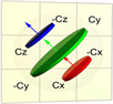Any vector $a+ib$ at the origin, when multiplied by i will preserve its length, while it is rotated by 90˚. Examples are shown in Figure 5.

Figure 5. One can choose any point on the torus (Kähler manifold) as the origin. (a) If the C-field is tangent to the surface in the direction $v_C$ , then the dual vector, $v_B=i{v}_C$ is rotated by π/2, retaining its magnitude and tangential nature. (b) If the C-field is multiplied by v then the dual vector, $v_B=-i{v}_C$ is rotated by 3π/2 or -π/2.

On a Kähler manifold, parallel-transporting a vector and then trans­forming it by the duality transformation is the same as duality transforming the original vector and then parallel-transporting it. Essentially, the C-field and its dual, the B-field, are always orthogonal and share the same parallel-transport properties.

In Figure 5 the y-axis is assumed to point locally in the direction of the core, circling the donut hole. The red C-field arrow, $v_C$ , has a component $v_{C_y}$ that circles the donut hole and another $v_{C_x}$ that circles the torus. In Figure 5(a) the blue B-field arrow, $v_B=i{v}_C$ , has a component $v_{B_y}$ that circles the donut hole in the same direction as the C-field, and another $v_{B_x}$ that circles the torus in the direction opposite to $v_{C_x}$ . In Figure 5(b) the blue B-field arrow, $v_B=-i{v}_C$ , has a component $v_{B_y}$ that circles the donut hole in the direction opposite to the C-field, while $v_{B_x}$ circles the torus in the same direction as $v_{C_x}$ . The C-field performs a U(1) × U(1)-rotation on the torus such that two 2π-rotations are required to return to the original state at the starting point, which, by virtue of the Kähler properties, can be any point on the torus. The B-field also performs a U(1) × U(1)-rotation on the torus. The Chern class vanishes, so there is no point on the manifold that will halt flow.

The C-field and its dual, the B-field, flow endlessly in this construction; this stable, self-organized field-structure.

i.e., the ontology of physical duality is such that the existence of the B-field implies the existence of electric charge current parallel to the C-field mass core current (momentum) induced by the self-linking toroidal solenoid of gravitomagnetic energy ultra-density distribution.

The C-field flow around the hole in the torus is determined by mass current $p$ . The B-field flows around the torus in the direction determined by the sign of the charge. Based on Figure 2, Figure 3, and Figure 5 we conclude that negative charge current ( $j=-qv$ ) induces left-handed B-field circulation, as $\nabla \times B=-qv$ is dual to mass current inducing C-field circulation, $\nabla \times C=-mv$ . The angular momentum of the field circulation is additive, as is the angular momentum around the donut hole. For positive charge B-field circulation is right-handed, yielding angular momentum of the B-field opposite to the C-field angular momentum. The helical C-field circulation is always left-handed, whereas the B-field helical circulation around the torus depends upon the sign of the charge and determines the direction of the magnetic moment $\mu$ in Figure 2(b). Intuitively, the maximum helical angular momentum around the torus, proportional to $\left(C\cdot C+B\cdot B\right)$ should be more stable than the minimum helical angular momentum, which is proportional to $\left(C\cdot C-B\cdot B\right)$ if the mass density of each field is proportional to the square of the field strength, but the contribution to angular momentum is proportional to the direction of the mass flow. If reasoning is valid, it might explain the predominance of electrons over positrons in the universe, a fact that has no explanation.

10. Flow of C-Field and B-Field

The result of our fermion charge genesis analysis consists of two circulating fields, dual to each other, with properties as described above. Figure 6 depicts three aspects of the same fermion. Figure 6(a) shows a translucent torus, enabling us to see the complete flow paths corresponding to dual points on the torus. Figure 6(b) shows the same flows on an opaque torus, such that only flows visible from one side can be seen. Figure 6(c) depicts the two flows translucently from an arbitrary perspective. Observe that from whatever perspective, when the B-field “crosses” the C-field, the apparent angle between the two is 90˚. Compare Figure 6 to Figure 1, which depicts the C-field flow derived from the Calabi-Yau spin analysis, corresponding to the red flow paths shown in Figure 6.

This is the Calabi-Yau-based primordial field theory of the origin of electric charge.

Figure 6. Three aspects of field flows on the same fermion. (a) translucent torus, (b) opaque torus, and (c) translucent torus from arbitrary perspective. In each figure the C-field is red, the B-field is blue.

11. Ontological Comparison of Charge Models

As there exist relatively few attempts to explain the origin of the electric charge, if the associated mathematics is reasonable, then comparison of such models will be based on ontological grounds.

Consider Faber’s model in which charges are introduced by adding a term with the finite structure constant $\alpha ~e^2$ to the Lagrangian, where proportionality symbol “~”, means that constant scale factors have been omitted. This mathematical introduction of charge is legitimate but does not physically “explain” the origin of charge. The model is based on an SO(3)-valued field that rotates in 3D space, which he calls the soliton field. Inspired by the Sine-Gordon model of topological fermions, he then introduces the idea of objects not connected to the environment, which return with 2π-rotation, and objects connected by wires to the surroundings, which require 4π-rotation to disentangle. This Dirac/Feynman “belt trick”, with no

known meaningful physical analogy, is often used as an example of spin- $\frac{1}{2}$ . He

claims that solitons transform to dual Dirac-magnetic monopoles with singularities enclosed and two-dimensional surfaces leading to the definition of electric charge:

$Q_s\left(s\right)=\frac{-e_o}{4\pi }{\displaystyle {\oint }_{S\left(u,v\right)}\text{d}u\text{d}vn\left[{\partial }_{\mu }n-{\partial }_{v}n\right]}$ (18)

He views electronic charge as a topological quantum number explaining the quantization of electric charge, with two charges, + and −, and concludes that mass is field energy and particles are topological solitons (although original solitons are implicitly in motion). His charges and their fields are not distinguishable; they are built from the same field, and he suggests that Maxwell’s theory is a clever way to get a linear theory from a nonlinear system, supporting non-topological magnetic currents [Dirac’s monopoles] that are unknown to Maxwell’s theory. In short, assumption of vortical structures and introduction of the fine structure constant lead to equations that can be interpreted as a non-separable [charged] particle/field. Faber’s equations of motion allow for magnetic monopole currents that are non-topological and act as sources of electric and magnetic fields. He speculates that non-topological currents escape the detectors, which thus measure only electric and magnetic fields, and finally notes that there are some ideas that could be worked out then compared with experiment. These ideas differ significantly from those in this paper and are largely rejected on ontological grounds.

Hans van Leunen views electrical charge as properties of space and formulates his model in terms of infinite dimensional separable quaternionic Hilbert space, wherein fields will appear as continuum eigenspaces of normal operators which map subspaces onto themselves. He focuses on “well-ordered normal operators” and starting with polar angle, then azimuth, and finally radius, notes that such spherical ordering may create a symmetry center. The 4D nature of the quaternion leads to well-ordered versions, half right-handed and the other half left-handed. Aspects of the 16 well-ordered versions are assigned to electric charge. Van Leunen says, “physical reality will show the features and phenomena of these structures”, effectively an “ontology free” approach to physical reality. While his mathematical model explains the origin of charge, it fails to explain the origin of ontological (physically real) electric charge in the universe.

12. Summary and Conclusions

I cannot overemphasize the degree to which I take ontology seriously. Many papers are published today in which something is posited that has never been seen, often formulated in dimensions that we cannot experience. These often rely upon either some analogy to physics, but sometimes only a pure mathematical analogy. For example, in quantum electrodynamics, every quantum force has a mediating quantum field, and each quantum field has its own particles. In QCD a pair of quarks bound into a pion are connected by a gluon field, often described as “a constant exchange of virtual gluons.” This is applied to Feynman diagrams where each pair of vertices represent interaction probabilities between particles, with the electromagnetic field emitting and absorbing a virtual photon. This is a handy calculational tool, but the virtual particles are not physically real.

As noted, the “quantum fields” of QED are particle-specific and based on the “mattress model” or harmonic paradigm. This basically boils down to the quantum theory of harmonic (raising and lowering) operators being applied statistically based on quantized energy. Most physical reality is based on equilibrium or systems moving toward equilibrium, so it is generally appropriate to formulate physics in a harmonic paradigm. Nevertheless, over the last century too many non-physical aspects have become embedded in physics, with the result being that things are so unreal that many physicists doubt the very existence of reality and think that the universe is made of math.

In the face of this, I attempt to start with ontological clarity and see how far this can be carried. It has been carried quite far, and here we hope to extend this to creation of electric charge in quantum gravity. It is difficult to say what most physicists mean by “quantum gravity”, as well proved in Armas’ Conversations on Quantum Gravity, but it often seems that it is based on a clear desire to reformulate gravity in the formulation of quantum mechanics. I have addressed this in “Ontology of Quantum Gravity”. What is meant here by quantum gravity is that the basis of quantum mechanics, de Broglie’s $p=\frac{h}{\lambda }$ both applies as derived in equation (5), that is, the gravitomagnetic field, induced by momentum density p, can be related to Planck’s constant and is effectively “quantized”. No other interpretation of quantum mechanics has been assumed.

A reviewer remarked that equations (8) look like two sets of dual field equations, but physically are not dual, because the electromagnetic field is a spin 1 particle, while gravity is a spin 2 particle. This is a significant criticism since duality is key to our derivation of electric charge. The claim is that lack of mathematical rigor leads to this kind of problem. First, I agree with Feynman that physics is not about mathematical rigor. My own belief is that often it is lack of ontological rigor that leads to problems. For example, the electric field in primordial theory is a “particle” (the photon) only in the sense that it represents localized stress in the field moving at the “speed of stress”, which is exactly the same speed as gravitomagnetic stress propagation. QED calls these localized stress waves “particles” and conceives of fields as a sea of such particles, as in the idea of “virtual particles” discussed above. Primordial field theory, instead, views the field as a continuum whose distribution defines space. Stress waves in this continuum have character associated with the duality of mass and charge. The generation of stress waves by negative q particles orbiting positive particle Q and the generation of stress waves by the dual of charge, i.e., mass m, orbiting another mass M are dual, and both are described by the primordial field equation. Thus spin-1 and spin-2 have significance when one believes fields are equivalent to a “sea of particles” but are ontologically dual aspects of the continuous primordial field, whereas spin- $\frac{1}{2}$ is ontologically real in the continuum model to which Calabi-Yau was applied.

A key term in primordial field theory is velocity v. Note for example that smoke rings are not static but consist of a flowing material layer while also moving through a local medium. So do “air rings” produced and played with by porpoises. The flow at the surface has velocity $v$ , which is a real speed of real “material”, the localized energy density of the field. $v$ is different from and less than the speed of stress waves in the field, which is the speed of light and the speed of gravity. Another key concept arising from primordial field theory is the complete absence of field strength, per se, in the derivation of the equations of motion. As a result, the theory is independent of field strength, depending instead upon mass density. The ultra-dense primordial field at the big bang induces ultra-strong fields, ignored by proponents of the “weak field approximation”. Ultra-turbulence is assumed at the big bang and hence vortices, helices, and tori.

Primordial theory has resolved most of the paradoxes associated with GR and has derived the Schwarzschild metric (an exact “static” solution of Einstein’s equation), the Kasner metric (an exact dynamic solution of Einstein’s equation) and has been used to reinterpret Michaelson-Gale’s experiment (1925), and the Tajmar Anomaly experiment (2006), and the Quantum Bouncer experiment (2000+), and others.

Summarizing, Yang-Mills self-interaction term, $\left[A^{\mu },A^{\nu }\right]$ , failed to solve the mass-gap problem, the gap between the lowest stable mass and the vacuum state. I restructured this self-interaction term to represent interactions between higher-order self-induced fields, then formulated these as path integrals on a fractal lattice to derive a stability theorem that yields a mass-gap existence proof. This stable torus is then analyzed as a Calabi-Yau manifold, and the U(1) × U(1) symmetry is shown to yield a structure with half-integral spin. Here we treat the origin of electric charge in terms of Jefimenko’s duality between Maxwell’s equations and Heaviside’s equations and conjecture the non-interacting co-existence of the torus induced by dual core source-flows. The resultant charge flowing in the core gives rise to the magnetic moment dual to the spin. Our treatment has thus yielded mass-gap, spin- $\frac{1}{2}$ , discrete charge, and magnetic moment.

Is this sufficient to calculate the mass from first principles? Other issues should be investigated before attempting to derive the mass. In our C-field-centric analysis, an increase in density seems “built-in” with no obvious limit in sight, necessitating the existence of the electromagnetic dual. Finally, we are interested in the “fractional” charge of the up and down quarks, and how their masses are affected by such. Once quarks have been analyzed, the issue of hadrons can be tackled.

In summary, we have not calculated the mass of the fermion generated by quantum gravity but have essentially derived a loop quantum gravity-based existence proof for a fermion, assuming the electron. To my knowledge no othertheory of loop quantum gravity has yielded the mass-gap, spin- $\frac{1}{2}$ , discretecharge, and magnetic moment of any fermion.

Appendix A: Galilean Transformation of Maxwell’s Equations

Phipps proved that field propagation through space is invariant under Galilean transformation if the total time derivative is used in Maxwell’s equations. This conflicts with Einstein’s claim of Lorentz transformation, based on his choice of the Maxwell-Hertz equation which he presented as the basic equation underlying special relativity:

$$\frac{1}{c}\frac{\partial E_x}{\partial t}=\frac{\partial B_z}{\partial y}-\frac{\partial B_y}{\partial z}$$ and $\frac{1}{c}\frac{\partial B_x}{\partial t}=\frac{\partial E_z}{\partial y}-\frac{\partial E_y}{\partial z}$ and permutations, (A.1)

Einstein claimed that one need not “assign a velocity-vector to a point of empty space in which electromagnetic processes take place”, contradicting Hertz’s assumption that “at every point a single definite velocity can be assigned to the medium which fills space.” Einstein’s theory is based on Maxwell-Hertz equations (A1) from Hertz’s first paper developing the theory of electromagnetics for bodies at rest; the correct equation (A2) is from Hertz’s paper on bodies in motion:

$$\frac{1}{c}\left[\frac{\text{d}B}{\text{d}t}+\left(v\cdot \nabla \right)B\right]=-\nabla \times E$$ and $\frac{1}{c}\left[\frac{\text{d}E}{\text{d}t}+\left(v\cdot \nabla \right)E\right]=-\nabla \times B+\frac{4\pi }{c}\rho v$ . (A.2)

These Maxwell-Hertz equations are invariant under Galilean transformation; from $r^{\prime }=r-vt$ and $t^{\prime }=t$ we find: ${\nabla }^{\prime }=\nabla$ , $\frac{\text{d}}{\text{d}{t}^{\prime }}=\frac{\partial }{\partial t}+v\cdot \nabla$ where $r^{\prime },t^{\prime }$ and $r,t$ specify coordinates of the same point in two relatively-moving “inertial” frames. The total time derivative is $\frac{\text{d}}{\text{d}t}=\frac{\partial }{\partial t}+v_e\cdot \nabla$ so applying Galilean law ${v^{\prime }}_e=v_e-v$ where $v_e$ is ether velocity measured in the unprimed (rest) frame, ${v^{\prime }}_e$ is the same measured in the primed frame, and $v$ is the (constant) velocity of the primed relative to the unprimed ( $v=0$ ) frame, we find

$\begin{array}{c}{\left(\frac{\text{d}}{\text{d}t}\right)}^{\prime }={\left(\frac{\partial }{\partial t}+v_e\cdot \nabla \right)}^{\prime }=\frac{\partial }{\partial t^{\prime }}+{v^{\prime }}_e\cdot {\nabla }^{\prime }\\ =\left(\frac{\partial }{\partial t}+v\cdot \nabla \right)+\left(v_e-v\right)\cdot \nabla =\frac{\partial }{\partial t}+v_e\cdot \nabla =\frac{\text{d}}{\text{d}t}\end{array}$ (A.3)

which verifies the first-order Galilean invariance of $\frac{\text{d}}{\text{d}t}$ . QED.

Phipps proved Galilean transformation invariance by substituting $\frac{\text{d}}{\text{d}t}$ in Maxwell’s equations; the term $\frac{\text{d}}{\text{d}t}=\frac{\partial }{\partial t}+v\cdot \nabla$ with $v$ the velocity of the media in which waves traverse the local gravitational field. Circa 1916 Einstein himselfrealized [letter to Lorentz] that the gravitational field supplied the “ethereal” medium, which he had built into his basic “inertial reference frame”. If local gravity is the medium of propagation, then the velocity of the lab frame with respect to this local ether is effectively $v=0$ ; Michelson and Morley did not disprove local ether; only that a universal isotropic homogeneous ether is invalid. In fact, of seven popular electromagnetic field theory texts (Jackson, Panofsky and Phillips, Lorraine and Corson, Wangness, Ohanian, Smythe, Purcell), all the authors address the problem of the partial derivative in Maxwell’s equations but explain it variously.

Appendix B: Retardation, Relativity, and Relativistic Mass

Retardation yields the equations of special relativity, while energy-time theory formulated in terms of (local) absolute space and universal time yields the relativistic Hamiltonian and clock slowing (aka “time dilation”) but not length contraction or Lorentzian velocity addition.

Heaviside’s equations derive from the primordial self-interaction equation, yet Jefimenko derives the same equations by replacing electromagnetic terms by corresponding gravitomagnetic terms; the identical results confirm the fundamental duality of electrodynamics and gravito-dynamics. Yet the physics of Maxwell and the physics of Heaviside differ enough to require further analysis. Many consider covariant formulation most appropriate for expressing laws of physics in a frame-independent form, given by the electro-magnetic 4-tensor, but Jefimenko reasoned:

“A covariant theory of gravitation is not possible unless the gravitational mass, just like the electric charge, does not depend on the velocity with which the mass moves. Until recently it was generally believed that the mass of a moving body was a function of the velocity of the body, and therefore was not invariant under relativistic transformation.”

This invariance was the most important reason to question the possibility of a theory of gravitation analogous to the theory of electromagnetics and Jefimenko suggests that this forced Einstein to create a theory of gravitation based not on the concept of the gravitational force field but on the concept of “curvature of space”. Yet neither gravitational nor inertial mass depends on the velocity with which a body moves, thus allowing construction of covariant gravity by substituting into electromagnetic structures, yielding primordial gravitomagnetic field tensor $F_{\mu \nu }$ [of equation (4)].

The value of a function placed between the retardation brackets is not that which the function has at the time t for which the integrals are evaluated, but that which it had at some earlier time $t^{\prime }=t-r/c$ ; the function is retarded. This reflects the reality that a time $r/c$ must elapse before the results of some event at the point $x^{\prime },y^{\prime },z^{\prime }$ can produce an effect at $x,y,z$ separated from point $x^{\prime },y^{\prime },z^{\prime }$ by a distance r.

Jefimenko did not discover retardation, but he appears to be the only one to derive all the fundamental equations of special relativity in a natural and direct way from the equations of the theory of electromagnetic retardation [22] , “without any additional postulates, conjectures, or hypotheses.” With retardation, none of the transformation equations obtained constitute actual equalities between the quantities involved, they “…are merely prescriptions for obtaining electric and magnetic potentials of a stationary charge distribution from the potentials of the same moving charge distribution by replacing quantities pertaining to the moving charge distribution by quantities pertaining to the stationary charge distribution and vice versa.”

I often use relativistic mass, $m=\gamma m_0$ in Energy-time theory, obviating the need for the Lorentz transformation on space and time. This is ontologically correct at the level of special relativity, which does not incorporate gravitation. When one adds primordial field theory to Energy-time theory then kinetic energy of the moving mass is shown to represent storage of energy in the C-field circulation, and mass is invariant. Today some physicists insist that “relativistic mass” is an invalid concept, while others, like Rindler [23] conclude that the idea of velocity dependent mass is a useful one. Steven Weinberg [24] points out that since $\text{d}\tau =\text{d}t/\gamma$ we obtain

$m\frac{\text{d}}{\text{d}t}\left[\gamma v\right]=q\left[E+\frac{v}{c}\times B\right]$ (B.1)

“It is a special feature of electromagnetic force that the only changes in the equation of motion introduced by special relativity is the replacement off mass m in the momentum with $m=\gamma m_0$ , [and thus] treat $\gamma m_0$ as a relativistic mass.”

In other words, unless and until one brings gravitomagnetic circulation energy into the picture, the concept of relativistic mass is conceptually useful.

Heaviside’s equations for the electric field of a point charge q moving with constant velocity v is relativistically correct and agrees with the same equation derived by Jefimenko from electro-magnetic retardation, implying that the equations are correct, while including length contraction in these derivations leads to incorrect equations. He concludes that length contraction is not physical [as does energy-time theory]. “Length contraction” was proposed by Lorentz in 1888 due to interaction of a moving body with the ether. In 1905 Einstein rejected ether but retained length contraction, but Jefimenko notes that length contraction requires two observers (two points of observation) and that the relativistically correct visual shape of a moving body is its retarded shape, concluding that as a physical phenomenon, relativistic length contraction does not exist.

Conflicts of Interest

The author declares no conflicts of interest regarding the publication of this paper.

References

[1]	Klingman, E. (2022) Journal of Modern Physics, 13, 1128-1145. https://doi.org/10.4236/jmp.2022.137065
[2]	Klingman, E. (2024) Journal of Modern Physics, 15, 132-158. https://doi.org/10.4236/jmp.2024.151005
[3]	Klingman, E. (2020) Journal of Modern Physics, 12, 65-81. https://doi.org/10.4236/jmp.2021.122007
[4]	Klingman, E. (2021) Journal of High Energy Physics, Gravity & Cosmology, 7, Article No. 3.
[5]	Faber, M. (2022) Journal of Physics, 361, Article ID: 012022. https://doi.org/10.1088/1742-6596/361/1/012022
[6]	Van Leunen, H. (2015) Open Access Library Journal, 2, e1836.
[7]	Heaviside, O. (1893) The Electrician, 31, 81-82.
[8]	Klingman, E. (2022) Journal of Applied Mathematics and Physics, 10, 2292-2302. https://doi.org/10.4236/jamp.2022.107156
[9]	Armas, J. (2021) Conversations on Quantum Gravity. Cambridge U Press, Cambridge. https://doi.org/10.1017/9781316717639
[10]	Yau, S. (2010) The Shape of Inner Space. Basic Books, New York.
[11]	Phipps, T. (2012) Old Physics for New: A Worldview Alternative to Einstein’s Relativity Theory. 2nd Edition, Apeiron, Montreal.
[12]	Hertz, H. (1890) Electric Waves “On the Fundamental Equations of Electromagnetics for Bodies in Motion”. Dover, Mineola.
[13]	Abbott, B., et al. (2017) Physical Review Letters, 119, Article ID: 161101. https://doi.org/10.1142/9789814699662_0011
[14]	Michelson, A. (1925) The Astrophysical Journal, 61, 137. https://doi.org/10.1086/142878
[15]	Klingman, E. (2020) Journal of Modern Physics, 11, Article No. 12. https://doi.org/10.4236/jmp.2020.1112123
[16]	Huang, K. (2007) Fundamental Forces… the Story of Gauge Fields. World Scientific, Hackensack. https://doi.org/10.1142/9789812770714
[17]	Jefimenko, O. (2000) Causality, Electromagnetic Induction & Gravitation. 2nd Edition, Electret Scientific Co., Star City, West Virginia.
[18]	Jackson, J. (1962) Classical Electrodynamics. John Wiley and Son, New York. https://doi.org/10.1063/1.3057859
[19]	Natsuume, M. (2014) AdS/CFT Duality User’s Guide. https://doi.org/10.1007/978-4-431-55441-7
[20]	Klingman, E. (2019) Prespacetime Journal, 10, 671-680. https://prespacetime.com/index.php/pst/article/view/1602
[21]	Sokolowski, L. (2016) The Bizarre Anti-de Sitter Spacetime.
[22]	Jefimenko, O. (1995) American Journal of Physics, 63, 267-272. https://doi.org/10.1119/1.17938
[23]	Rindler, W. (1991) Introduction to Special Relativity. 2nd Edition, Oxford Science Pub, Oxford.
[24]	Weinberg, S. (2021) Foundations of Modern Physics. Cambridge U. Press, Cambridge, 121. https://doi.org/10.1017/9781108894845