Effects of Chlorine and Chlorine Monoxide on Stratospheric Ozone Depletion

Laurie Wei, Ibraheem Alelmi, Sen Nieh^*

Department of Mechanical Engineering, The Catholic University of America, Washington, DC, USA.

DOI: 10.4236/acs.2024.141009                

Abstract

This paper presents a system approach of mass balance calculations of ozone and other species under diffusion-convection-reaction processes to study the impacts of major ozone-depleting chemicals, chlorine (Cl) and chlorine monoxide (ClO), and the effect of photolysis on ozone concentrations, ozone depletion, total ozone abundance, and ozone layer along the altitude in the stratosphere. The calculated ozone concentrations and profile of the layer followed a similar trend and were generally in good agreement with the measurements above the tropical area. The calculated peak of the layer was at the same mid-stratosphere at Z = 30 km with a peak concentration and total ozone abundance about 20% higher than the measured peak concentration of 8.0 ppm and total abundance of 399 DU. In the presence of Cl and ClO, the calculated ozone concentrations and total abundance were substantially reduced. Cl generally depleted more uniformly of ozone across the altitude, while ClO reduced substantially the ozone in the upper stratosphere and thus shifted the peak of the layer to a much lower elevation at Z = 14 km. Although both ClO and Cl are active ozone-depleting chemicals, ClO was found to have a more pronounced impact on ozone depletion and distribution than Cl. The possible explanations of these interesting phenomena were discussed and elaborated. The approach and calculations in this paper were shown to be useful in providing an initial insight into the structure and behavior of the complex ozone layer.

Keywords

Ozone, Ozone Depletion, Chlorine, Chlorine Monoxide, Photolysis, Dobson Unit

1. Introduction

1.1. Distribution of Stratospheric Ozone

Being presented in small trace amounts, stratospheric ozone is good and very important to human health and environmental stability as a protective layer to absorb the harmful high ultraviolet (UV) rays. However, small amount of ozone in the troposphere near the ground is known to be polluting photochemical smog, being bad for the human, living beings, and the ecosystem [1] . Ozone is depleted and destroyed when it meets and reacts with chlorine- or bromine-containing chemicals and nitrogen compounds, which is why traditional refrigerants used in HVAC and refrigeration, such as chlorofluorocarbons (CFCs) and hydrochlorofluorocarbons (HCFCs) being regarded as ozone depleting substances for reducing stratospheric ozone.

Both CFCs and HCFCs have carbon, chlorine, and fluorine while HCFCs have hydrogen and CFCs do not. Depending on the amount of chlorine in the refrigerants, their ozone depletion potentials would be different. For instance, traditional refrigerant CFC-12 (or dichlorodifluoromethane CF₂Cl₂) contains two chlorines and 59% by mass in the refrigerant, which is higher than refrigerant HCFC-22 (or chlorodifluoromethane CHF₂Cl) of one chlorine and 41% by mass. CFC-12 will release more reactive Cl and cause more depletion of ozone than HCFC-22 in the stratosphere. Additionally, CFCs can stay in the stratosphere for as long as 130 years. A longer atmospheric lifetime of CFCs than HCFCs would deliver more reactive Cl and consume more ozone than HCFCs in the stratosphere.

In the 1980s, scientists M.J. Molina and F.S. Rowland worked under P. Crutzen discovered the ozone hole and the link of chlorofluoromethane to the hole size based on their laboratory tests and computational modeling, which led to the Nobel Prize in Chemistry in 1995 [2] . The stratospheric ozone distribution across the globe varies with the geographical location, altitude, time and season of the year, and the presence of ozone-depleting chemicals. The total ozone column above a location varies typically from 200 to 500 Dobson Units (DU) with a global average of 300 DU [3] .

A general mass balance equation will be used to account for the interactions of convection, diffusion and various chemical processes to focus on the study of ozone distribution and depletion. Ozone behavior and dynamics in the stratosphere are basically characterized by five competing chemical-physical processes: photolysis, diffusion, convection, ozone generation reactions, and ozone depleting reactions. Various theoretical and numerical models were developed, such as the general mass balance equations, to account for the interactions of convection-diffusion-chemical reactions. While the modeling is an ongoing, multidimensional approach to studying ozone behavior and man-made depletion, the results discussed in this paper are of the effects of chlorine, chlorine monoxide, and photolysis (time of the day) on ozone concentrations in the tropical area. The purpose of this research is to characterize and quantify, when possible, the influence of major ozone depleting chemicals and factors on ozone concentrations, depletion, and profile of the layer in the stratosphere.

1.2. Refrigerants and Ozone Depletion

Mankind today relies heavily on air conditioning and refrigeration for daily needs, with about 2 billion ACs and 1.4 billion refrigeration units in the world. Megatonnes of chlorine-containing chemicals were emitted into the atmosphere in the world per year in the late 20^th century. Two types of global atmospheric effects are involved in air conditioning and refrigeration: 1) the global warming potential (GWP) due to the atmospheric greenhouse effect from some refrigerant gases, and 2) ozone depleting potential (ODP), due to the emission of chlorine-containing refrigerants [4] [5] . Traditional refrigerants of CFCs and HCFCs have exceptional stability, allowing them to survive in the atmosphere for decades.

Refrigerants have evolved since the 1800s and CFCs were welcomingly introduced in 1928, known to be a series of safe, stable, good refrigeration performance, and economical refrigerants until their damaging effects on the ozone layer were discovered in the 1970s. Zero or low ODP and zero or low GWP became desired performance characteristics to the point since the searches for alternatives to CFCs and HCFCs began in the 1970s [6] . In 1995, Rowland and Molina discovered the link between CFCs and ozone depletion, proposing an equation ${\text{O}}_2+\text{light}\to 2\text{O}$ and $\text{O}+{\text{O}}_2+\text{M}\to {\text{O}}_3+\text{M}$ with M being a random air molecule such as N₂ and O₂ [7] . The photo-dissociation reaction rates in the stratosphere were modeled and calculated after Kockarts [8] and Brinkmann [9] for an averaged value, globally for diurnal and zenith angle effects.

1.3. Ozone-Depleting Chemicals—Chlorine, and Chlorine Monoxide

Gases such as refrigerant vapors, methane (CH₄), nitrous oxide (N₂O), chlorine Cl, and chlorine monoxide ClO are known to be ozone-depleting chemicals. The main perpetrators are known to be chlorine-containing halogen source gases from various CFCs and HCFCs molecules, which form reactive halogen gases of Cl and ClO in the stratosphere under the sunlight with an intense high-energy UV. CFCs and HCFCs have been used widely in many applications, including refrigeration, air conditioning, foam blowing, spray can propellants, and cleaning of metals and electronic components. Reactive chlorine gases Cl and ClO were observed and measured in the stratosphere using both local and remote measurement techniques [6] . In the troposphere, chlorine-containing source gases emitted by human activities are chemically stable, undergo little or no loss, and accumulate, until transported to the stratosphere by air motions. In the ozone layer in the stratosphere (10 km - 50 km), the amount of source gases gradually declines while the reactive chlorine gases increase [6] .

Changes in solar radiation and reactive chlorine gases in the stratosphere affect the abundance of stratospheric ozone, with higher chlorine levels leading to lower abundances of ozone and lower solar radiation in the stratosphere. Values of Equivalent Effective Stratospheric Chlorine (EESC) were derived from surface observations to show the potential of ozone depletion in the stratosphere, with higher levels of EESC being more closely associated with long-term ozone depletion. Total ozone is least affected in the equator and tropics (20˚N - 20˚S) and most affected in the poles, due to large-scale atmospheric transport where air entering the equatorial region and moving pole-ward in both hemispheres in the mid-to high-latitudes before returning to the troposphere. However, a high solar UV radiation in the equator causes a net ozone production in the tropics. Chlorine monoxide ClO is known to be the most reactive chlorine gas that destroys stratospheric ozone in a chlorine catalytic cycle for ozone depletion [6] . The total ozone column above a geographical location varies from 200 to 500 Dobson Units (DU), with ozone generation from solar UV radiation in tropical areas being the strongest. However, the total ozone is reportedly a smaller value above the equator and larger values in the mid-latitudes and the polar region, because of the slow, large-scale horizontal circulation of ozone-rich stratospheric air taken from the tropical areas [1] [6] .

To better understand the observational data of ozone distribution and depletion, different modeling efforts were conducted [1] [10] [11] . An earlier model was the photochemical box model simulating the transport and chemistry of ozone depletion. 2-D and 3-D models, such as latitude-altitude models and zonal mean models, focusing more on in-depth study for solving atmospheric species kinetics and circulation-related issues have gained attention in recent years [10] [11] . These models may offer a more thorough knowledge of different atmospheric gas species. However, while they provide a chemically based model for convection and diffusion, they may not show a focus on ozone behavior and distribution. It is of interest to combine the calculated results with observational/measured data to fully comprehend the dynamics and behavior of the ozone layer.

In this paper, we use general mass balance equations to account for the ozone-related interactions of convection-diffusion-chemical reactions to focus on the study of ozone concentration, distribution and depletion. Although the modeling is an ongoing, multi-dimensional approach, the results discussed in this paper are of 1-D model and calculations, with major atmospheric properties and physical-chemical processes being only a function of altitude. It’d be easier to interpret the complex results of ozone dynamics under specific conditions, as compared to the measured data, with or without Cl and ClO, at noontime in the tropical areas [1] [10] . This approach provides a higher resolution along the vertical structure of the atmosphere and the detailed processes along the altitude. It is computationally efficient and believed to be useful in providing an initial insight into the complex dynamics of the ozone layer and depletion.

2. Modeling and Numerical Methods

2.1. Mass Balance Equations

The Mass Balance Equations in Equations (1) and (2) below, involving five competing physical-chemical processes: wind convection, mass diffusion, dynamic change, ozone generating reactions, and ozone depleting reactions, were used to model and calculate ozone O₃ and atomic oxygen O concentrations [1] . Since partial pressure and concentrations of molecular oxygen O₂ are stable and very large with an existing amount of 20.95% of air, the mass balance equation for molecular oxygen O₂ can be safely dropped because of the changes of O₂ will be negligibly small, as compared to changes of ozone and atomic oxygen.

$\begin{array}{l}\frac{\partial \left[\text{O}\right]}{\partial t}+u\frac{\partial \left[\text{O}\right]}{\partial z}-D_{\text{O}}\frac{\partial \text{O}}{\partial z^2}=\frac{\text{d}\left[O\right]}{\text{d}t}\\ =k_1\left[\text{O}\right]\left[{\text{O}}_{\text{2}}\right]-k_2\left[\text{O}\right]\left[{\text{O}}_{\text{3}}\right]+k_3\left[{\text{O}}_{\text{2}}\right]+k_4\left[{\text{O}}_{\text{3}}\right]-k_7\left[\text{ClO}\right]\left[\text{O}\right]\end{array}$ (1)

$\begin{array}{l}\frac{\partial \left[{\text{O}}_{\text{3}}\right]}{\partial t}+u\frac{\partial \left[{\text{O}}_{\text{3}}\right]}{\partial z}-D_{{\text{O}}_{\text{3}}}\frac{{\partial }^2\left[{\text{O}}_{\text{3}}\right]}{\partial z^2}=\frac{\text{d}\left[{\text{O}}_3\right]}{\text{d}t}\\ =k_1\left[\text{O}\right]\left[{\text{O}}_{\text{2}}\right]-k_2\left[\text{O}\right]\left[{\text{O}}_{\text{3}}\right]-k_4\left[{\text{O}}_{\text{3}}\right]-k_5{\left[{\text{O}}_{\text{3}}\right]}^2-k_6\left[\text{Cl}\right]\left[{\text{O}}_{\text{3}}\right]\end{array}$ (2)

Finite difference equations along the altitude Z were derived, with derivatives of atomic oxygen [O] concentration and ozone concentration [O3] given below:

${\left[\text{O}\right]}^{\prime }=\frac{{\left[\text{O}\right]}_{i-1}-{\left[\text{O}\right]}_{i+1}}{2\Delta Z}=\frac{\partial \left[\text{O}\right]}{\partial z}$ , ${\left[\text{O}\right]}^{\prime \text{}\prime }=\frac{{\left[\text{O}\right]}_{i-1}-2{\left[\text{O}\right]}_i+{\left[\text{O}\right]}_{i+1}}{{\left(\Delta Z\right)}^2}=\frac{{\partial }^2\left[\text{O}\right]}{\partial z^2}$ and ${\left[{\text{O}}_{\text{3}}\right]}^{\prime \text{}\prime }=\frac{{\left[{\text{O}}_3\right]}_{i-1}-{\left[{\text{O}}_3\right]}_{i+1}}{2\Delta Z}=\frac{{\partial }^2\left[{\text{O}}_3\right]}{\partial z^2}$ . A MATLAB code was developed and used in

the calculations. Nonlinear terms in Equations (1) and (2), such as $k_2\left[\text{O}\right]\left[{\text{O}}_{\text{3}}\right]$ , were solved by successive approximation iterations, where initial values of [O] and [O3] were first guessed, and gradually modified according to the new values calculated in the previous run, till the difference between the two runs converged to an acceptably small value. Ozone-depleting catalytic reactions of chlorine Cl and chlorine monoxide ClO were considered, as characterized by reaction rate constants in Table 1(b): k₆ (= 2.16 × 10⁻³²) and k₇ (=8.53 × 10⁻¹⁵), respectively [1] . Assuming a steady state condition, or $\frac{\partial }{\partial t}=0$ , Equations (1) and (2) describe simultaneous algebraic finite difference equations of the mass balance of O and O₃, with the boundary conditions and parameters based on practical considerations and selections, as well as by Salawitch et al. [1] [6] .

2.2. Ozone Producing and Depleting Equations

Table 1(a) and Table 1(b) list a total of seven ozone producing and depleting reaction equations and the nominal values of reaction rate constants: k₁, k₃ of Equations (3) and (4), and k₂ and k₄ - k₇ of Equations (5)-(9) [1] . The reaction rate constants k₁, k₂, and k₅ depend greatly on the activation energies of O, O₂ and O₃ and temperature of the stratospheric air, while k₃ and k₄ depend on solar UV beams at different times of the day and months of the year. The seven reaction equations in Table 1(a) and Table 1(b), convection of slow air motion, and diffusion from concentration gradients, lead to increases or decreases in ozone and atomic oxygen concentrations and partial pressures in the stratosphere. Aside from altitude Z, parameters such as time of day affecting constants k₃ and k₄, boundary values of chlorine and chlorine monoxide, wind speed u, and diffusivities of gases were taken from the published data of measurements at a given Table 1. (a) Ozone-producing equations and nominal value of reaction rate constants, k₁ and k₃, of Equations (3) and (4) [1] [10] ; (b) Ozone-consuming equations and nominal value of reaction rate constants, k₂ and k₄ - k₇, of Equations (5)-(9) [1] [10] .

location [1] [10] .

Equations (8) and (9) show the reactions occurring in a chlorine catalytic cycle. Chlorine is considered an ozone-depleting catalyst since chlorine (Cl) and chlorine monoxide (ClO) are reformed after the completion of each cycle, which can be used again for further destruction of ozone. Three different principal reaction cycles are involved in the formation of Cl and ClO, with the first ozone destruction cycle being $\text{Cl}+{\text{O}}_3\to \text{ClO}+{\text{O}}_2$ and $\text{ClO}+\text{O}\to \text{Cl}+{\text{O}}_2$ [6] , with Cl and its derivative ClO serving as a catalyst and the overall reaction to be Equation (5), $\text{O}+{\text{O}}_3\to 2{\text{O}}_2$ . This is the first and most important cycle in the tropical area and mid-latitudes of Earth, with more intense solar radiation containing UV, including the high energy UV-C radiation above 30 km that breaks molecular oxygen into reactive atomic oxygen in Equation (4). During the entire time of its stay as catalyst in the stratosphere, a chlorine atom can deplete and destroy many thousands of ozone molecules [6] .

Cycle 2 and Cycle 3 [6] are primarily for polar ozone destruction, both forming an overall reaction of Equation (7), $2{\text{O}}_3\to 3{\text{O}}_2$ , with the involvement of chlorine Cl, bromine Br, and their ozone-depleting derivatives, where solar radiation (UV beam) is needed to break apart molecules such as ClO and BrCl. Cycle 2 starts from the reaction of two ClO to form (ClO)_2, and photolyzed into Cl and ClOO. Cl then reacts with O₃ into O₂ and ClO. Cycle 3 starts with the reaction of ClO and BrO, to form ClBr, and photolyzed into Cl and Br. Cl and Br then react with O₃ and ClO and BrO, resulting a net overall reaction of $2{\text{O}}_3\to 3{\text{O}}_2$ . Such cycles won’t occur in the dark and are most active when sunlight with energetic UV-C rays returns to the polar region [6] . For an initial study of complex dynamics and behavior of the stratospheric ozone layer, we consider only Cycle 1 for most geographical locations on Earth except for polar zones in this paper.

3. Results of Ozone Concentrations and Profile

Ozone O₃ is a tri-atomic gas naturally present in the stratosphere. It has a pungent odor that can be detected even at very low amounts. Ozone was first discovered in laboratory experiments in the mid-1800s, and its presence in the atmosphere was measured using chemical and optical methods in the mid-1900s [6] . It can react with many chemicals and can be explosive in concentrated amounts. Electrical discharges are generally used to produce ozone for industrial processes, such as air and water purification and bleaching of textiles and food products.

The ozone layer and distributions along the altitude in the stratosphere above the tropical area were calculated and compared to the published measured data in an earlier paper. The peak ozone layer was calculated to be 9.7 ppm in the mid-Stratosphere around 30 km, and the calculated ozone distribution exhibited a similar profile to the observational data with a standard deviation of the differences of 0.25 [1] .

3.1. Chlorine and Chlorine Monoxide

Calculated ozone concentrations in ppm with different amounts of chlorine (Cl) or chlorine monoxide (ClO) along the altitude of the stratosphere (10 km to 50 km), measured and calculated ozone concentrations without Cl and ClO, are listed in Table 2, along with the total ozone abundance (weighted area enclosed by the curve and the y-axis of altitude) in Dobson Units (DU). The measured concentrations of atomic oxygen [O] and ozone [O3] along the altitude Z, with or without Cl and ClO, use the literature values [Cl] = 3.80 × 10⁻¹² ppm and [ClO] = 6.17 × 10⁻⁹ ppm from Chakrabarty et al. [12] . The boundary conditions of both atomic oxygen [O] and ozone [O3] concentrations at the bottom of the stratosphere (Z = 10 km) were taken to be 0.4 ppm, and at the top of the stratosphere (Z = 50 km) to be [O] = 1.5 ppm and [O3] = 2.5 ppm, respectively.

From the data in Table 2, Figures 1 and 2 plot the ozone concentrations and distributions along the altitude Z, with or without chlorine [Cl] and chlorine monoxide [ClO]. Figure 1 shows a comparison between the measured (green curve) and calculated (yellow curve) ozone distributions above the equator at noontime, with neither [Cl] nor [ClO] presence in the Stratosphere. As seen, in the entire stratosphere from 10 km to 50 km, the calculated ozone distribution displayed a similar profile and trend to the observational data, with the peak of the ozone layer appearing around 30 km.

As shown in the figures, the calculations were higher than the measurements near the peak of the ozone layer in the mid-stratosphere, but were in good agreement with the measurements in the lower and upper stratospheres. As listed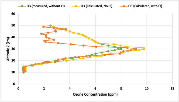

Figure 1. Comparison between the measured and calculated ozone distributions above the equator with no [Cl] or [ClO] in the stratosphere, and the calculated zone distribution with [Cl] = 3.8 × 10⁻¹² ppm and [ClO] = 0.

Table 2. Calculated ozone concentrations with chlorine (Cl) or chlorine monoxide (ClO), measured and calculated ozone concentrations without Cl and ClO, and the total ozone abundance (area) in Dobson Units (DU).

in Table 2, the calculated total ozone abundance without the presence of Cl and ClO is 479 DU, which is about 20% larger than the measured total ozone abundance of 399 DU.

The comparison of the calculated ozone distributions, without the presence of [Cl] (yellow curve) and with a literature value of [Cl] = 3.8 × 10⁻¹² ppm (orange curve) above the equator at the noontime, showed the same trend and good agreement in the lower stratosphere of Z < 30 km. But the presence of [Cl] in the upper stratosphere substantially reduces the ozone concentration, particularly in the zone of 35 km > Z > 45 km. It is believed that the UV radiation and thus the atomic oxygen concentration are much stronger and larger in the upper Stratosphere, which favors the catalytic reactions for ozone depletion, shown in Equations (8) and (9) in Table 1(b).

Figure 2 showed comparison of the calculated ozone concentrations in ppm along the altitude Z above the equator under the same boundary conditions and value of parameters for three cases of [Cl] = 0 and [ClO] = 0 (blue curve), [Cl] = 3.8 × 10⁻¹² ppm and [ClO] = 0 (orange curve), and [Cl] = 0 and [ClO] = 6.16 × 10⁻⁹ ppm (gray curve). The ozone distribution profile (gray curve) in the presence of chlorine monoxide (ClO) was quite different in the entire stratosphere from that (orange curve) in the presence of chlorine (Cl), which exhibited similar trend in the lower stratosphere but not in the upper Stratosphere in ozone distribution with the profile (blue curve) of no ozone depleting chemicals, Cl and ClO.

Figure 3 and Figure 4 show the results of sensitivity study of ozone-depleting chemicals, chlorine Cl and chlorine monoxide ClO, on ozone concentrations and distributions in the Stratosphere. Figure 3 includes two groups of curves at six different chlorine concentrations: [Cl] = 3.8 × 10⁻³ ppm, 3.8 × 10⁻⁴ ppm, and 3.8 × 10⁻⁵ ppm for a higher concentration than the literature value of [Cl] = 3.8 × 10⁻¹² ppm [12] , and [Cl] = 3.8 × 10⁻¹² ppm, 3.8 × 10⁻¹⁴ ppm, and 0 ppm for a lower value than the literature value or zero concentration.

As seen at the bottom of Table 2, the total ozone abundance in the Stratosphere has substantially reduced in the presence of Cl from 479 DU for zero [Cl], to 408 DU for [Cl] = 3.8 × 10⁻¹² ppm and [Cl] = 3.8 × 10⁻¹⁴ ppm, to 380 DU for [Cl] = 3.8 × 10⁻⁵ ppm, to 238 DU for [Cl] = 3.8 × 10⁻⁴ ppm, to 59 DU for [Cl] =

Figure 2. Comparison of the calculated ozone concentrations in ppm along the altitude Z above the equator for three cases of [Cl] = 0 and [ClO] = 0, [Cl] = 3.8 × 10⁻¹² ppm and [ClO] = 0, and [Cl] = 0 and [ClO] = 6.16 × 10⁻⁹ ppm.

Figure 3. Effects of amount of chlorine Cl on stratospheric ozone concentrations and distribution: two groups of curves at 6 different chlorine concentrations, [Cl] = 3.8 × 10⁻³ ppm, 3.8 × 10⁻⁴ ppm, and 3.8 × 10⁻⁵ ppm (higher concentration), and [Cl] = 3.8 × 10⁻¹² ppm, 3.8 × 10⁻¹⁴ ppm, and 0 ppm (lower concentrations).

Figure 4. Effects of amount of chlorine monoxide ClO on stratospheric ozone concentrations and distribution: a family of curves at 6 different ClO concentrations, [ClO] = 6.17 × 10⁻⁶ ppm, 6.17 × 10⁻⁷ ppm, 6.17 × 10⁻⁹ ppm, 6.17 × 10⁻¹⁰ ppm, 6.17 × 10⁻¹¹ ppm, and 0 ppm.

3.8 × 10⁻³ ppm. It is noted that one Dobson Unit (1 DU) represents the number of molecules required to create pure ozone of 0.01 mm column thick at the sea level of temperature 0˚C and pressure of 101 kPa (or 1 atm) [12] [13] . Since the temperature T, pressure P, and density ρ of air decrease drastically as it ascends from the ground level (Z = 0) to the bottom (Z = 10 km), the middle (Z = 30 km), and the top (Z = 50 km) of Stratosphere, the total ozone abundance in Dobson Unit at a geological location can be integrated from the weighted average of [O3] curve in ppm over T, P, and ρ along the altitude Z (from 10 km to 50 km), using a working formula $\text{DU}=\frac{{\left[{\text{O}}_3\right]}_{\text{ppm}}\left[\left(6.022\times {10}^{23}\right)\left(\frac{P}{RT}\right)\right]}{2.69\times {10}^{19}}$ .

Based on the literature value of ClO of 6.17 × 10⁻⁹ ppm [12] , Figure 4 shows the impact of chlorine monoxide ClO in the Stratospheric on ozone concentrations and distribution for six different values: [ClO] = 6.17 × 10⁻⁶ ppm (×1000, red curve), 6.17 × 10⁻⁷ ppm (×100, gray curve), 6.17 × 10⁻⁹ ppm (the literature value), 6.17 × 10⁻¹⁰ ppm (×0.1), 6.17 × 10⁻¹¹ ppm (×0.01), and zero concentration (blue curve). For the five cases of [ClO] > 6 × 10⁻¹¹ ppm, the ozone profiles were crowded together with a low ozone concentration close to the boundary value of 2.5 ppm, and also the profile changed to a quite different shape from the green curve. Not only the magnitude and shape of ozone curves changed substantially, the peaks of ozone layer shifted from the mid-stratosphere (Z = 30 km, blue curve) for zero ClO towards the bottom of the Stratosphere at Z = 12 - 16 km, when ClO presented with different amounts.

Although both chlorine Cl and chlorine monoxide ClO in the Stratosphere act as a catalyst to deplete the ozone, ClO was found to cause more pronounced impact than Cl. The impact of chlorine Cl on ozone concentrations and the total abundance was substantial and clear; however, its impact on ozone distribution profile and the peak location of ozone layer was not evident.

3.2. Photolysis

The reaction rate constants k₃ in Equation (4) of Table 1(a) and k₄ in Equation (6) of Table 1(b) depend on the strength of high energy UV beam at different times of the day and at different months of the year, which is referred to as the photolysis process. The variations of k₃ and k₄ with time of the day or the location of the Sun in the sky were modeled by J. Makungu et al. [10] $k_3={\text{e}}^{\frac{c_3}{\sin \left(\omega t\right)}}$ and $k_4={\text{e}}^{\frac{c_4}{\sin \left(\omega t\right)}}$ , where $c_3=22.62$ , $c_4=7.601$ , and $\omega =\frac{\pi }{43200s^{-1}}$ . Such values of k₃ and k₄ rise rapidly at dawn (t = 0, or depending on the month of the year), reach a peak at noon (t = 6), and decrease to zero at sunset (t = 12) [10] . As seen in Table 3, the values of k constant may depend on time of the day, altitudes at peak ozone concentrations, and the area between the ozone curve and altitude Z axis. Figure 5 shows the variation of photolysis reaction constants k₃ and k₄ with time in the day above the tropical area. The curves are symmetric about the noontime at 12:00 pm and become effectively zero before the dawn and after the dusk in a day.

Figure 5. Variation of photolysis reaction constants k₃ of Equation (4) and k₄ of Equation (6) with time or the motion of Sun in the day above the tropical area.

Figure 6. Effect of photolysis at different times of the day on ozone concentrations and distributions in the stratosphere above the tropical area.

Figure 6 plots the effect of photolysis at different times of the day on ozone concentrations and distributions in the stratosphere above the tropical area. As seen in Figure 6 and also Table 3, in the early morning at 7 am or late afternoon at 5 pm, the photolysis is weak with $k_3=1.06\times {10}^{-38}$ and $k_4=1.74\times {10}^{-13}$ for

Table 3. List of values of reaction constant k₃ in Equation (4) and k₄ in Equation (6) for photolysis of the solar beams, depending on time of the day in the tropical zone, and the calculated area between the ozone profile and altitude axis Z, and the total ozone abundance in Dobson units (DU).

Equations (4) and (6).

4. Discussions

4.1. Effects of Chlorine and Chlorine Monoxide on Ozone Distribution

From the data in Table 2, Figure 1 and Figure 2 plot the ozone concentrations and distributions along the altitude Z, with or without chlorine [Cl] and chlorine monoxide [ClO]. Figure 1 shows a comparison between the measured (green curve) and calculated (yellow curve) ozone distributions above the equator at noontime, with neither [Cl] nor [ClO] presence in the Stratosphere. As seen, in the entire stratosphere from 10 km to 50 km, the calculated ozone distribution displayed a similar profile and trend to the observational data, with the peak of the ozone layer appearing around 30 km.

As shown in Figure 1, the calculations were higher than the measurements near the peak of the ozone layer in the mid-stratosphere, but were in good agreement with the measurement in the lower and upper stratospheres. As listed in Table 2, the calculated total ozone abundance without the presence of Cl and ClO is 479 DU, which is about 20% larger than the measured total ozone abundance of 399 DU.

The comparison of the calculated ozone distributions, without the presence of [Cl] (yellow curve) and with a literature value of [Cl] = 3.8 × 10⁻¹² ppm (orange curve) above the equator at the noontime, showed the same trend and good agreement in the lower stratosphere of Z < 30 km. But the presence of [Cl] in the upper stratosphere substantially reduces the ozone concentration, particularly in the zone of 35 km > Z > 45 km. It is believed that the UV radiation and thus the atomic oxygen concentration are much stronger and larger in the upper Stratosphere, which favors the catalytic reactions for ozone depletion, shown in Equations (8) and (9) in Table 1(b).

In the presence of chlorine monoxide ClO, the ozone concentration spiked sharply from the bottom of the Stratosphere to 13 ppm around Z = 12 km, which is near the tropopause and stratosphere. However, instead of increasing, the further it gets into the stratosphere above Z = 15 km, the ozone concentration levels started decreasing rapidly and approached gradually the low boundary value of [O3] = 2.5 ppm in the upper Stratosphere. The ozone-depleting characteristics in the presence of chlorine monoxide (ClO) make the ozone profile peak at a much lower elevation (Z < 15 km), as distinctly opposed to the profile without the presence of ClO, peaking at Z = 30 km. Chlorine monoxide ClO evidently caused a more pronounced impact on ozone depletion than chlorine Cl.

As seen in Figure 3, the amount of chlorine [Cl] in the Stratospheric caused a significant impact to the ozone concentrations, distributions, and the total ozone abundance. Without the presence of Cl (blue curve), the ozone concentration was high, with a peak value of 9.7 ppm at Z = 30 km and a total abundance of 479 DU. As the amounts of Cl increased (yellow, orange, red, and green curves), the ozone concentrations and distributions decreased to a different degree, but more in the upper Stratosphere. However, the ozone peak locations remained at the mid-stratosphere around Z = 30 km. The impact of Cl on reducing the stratospheric ozone concentrations seems to be more uniform, with similar ozone layer profiles in the presence of different values of [Cl].

It is of interest to note that as the amount of Cl increased beyond a critical value of [Cl] = 3.8 × 10⁻⁴ ppm (such as at 3.8 × 10⁻³ ppm, deep blue curve), the depletion of ozone would be strong and evident, the peak ozone concentration would substantially reduce to close to half, or 5.2 ppm for [Cl] = 3.8 × 10⁻⁴ ppm, and to a much small value of 1.1 ppm for [Cl] = 3.8 × 10⁻³ ppm. The distribution profiles of ozone seem to remain the same trend with similar shapes. The total ozone abundance of the measured value was 399 DU, and the calculated value was 479 DU without the presence of Cl nor ClO, 408 DU with no ClO but with [Cl] = 3.8 × 10⁻¹² ppm, and 124 DU with no Cl but with [ClO] = 6.16 × 10⁻⁹ ppm. The difference between the calculated and measured values was +80 DU, or 20 %. The impact of the presence of [Cl] at the literature value was 408 DU over 479 DU, or −71 DU (reduction of 15% of total ozone). The impact of the presence of [ClO] at the literature value was 124 DU over 479 DU, or −355 DU (reduction of 74 % of total ozone). Higher concentrations of ozone-depleting chemicals, Cl and ClO, in the stratosphere, should lead to even lower total ozone abundance DU levels. The impact of ClO was found to cause more pronounced reduction of ozone than Cl.

The impacts of chlorine monoxide ClO on ozone concentrations, the total ozone abundance, the distribution profile, and the peak location of ozone layer were all substantial, clear, and evident. It may be discussed and understood from the depletion reaction equations in Equation (8), $\text{Cl}+{\text{O}}_3\to \text{ClO}+{\text{O}}_2$ , and Equation (9), $\text{ClO}+\text{O}\to \text{Cl}+{\text{O}}_2$ . Chlorine Cl can deplete an existing ozone molecule into a regular oxygen molecule and chlorine monoxide ClO, which then combines with an atomic oxygen O to revert back to chlorine Cl and another regular oxygen molecule. The depleting impact of Cl depends on the concentration of ozone [O3], while the depleting impact of ClO depends on the concentration of atomic oxygen [O]. The concentration of [O] is generated from photolysis of UV beams in the Stratosphere, whose intensity deteriorates as it penetrates into the air mass of the stratosphere. The weakened concentration of [O] in the lower Stratosphere [1] reduces the ozone depleting effect of ClO, as in Equation (9).

4.2. Effect of Photolysis

The change in peak of ozone layer, from that of the noontime 12:00 pm of the strongest Sun, shifts about 9 km toward the upper Stratosphere, with the highest ozone concentration of 9.07 ppm at Z = 39 km. At 9 am or 3 pm of the day, the photolysis becomes stronger and the change in peak of ozone layer shifts about 8 km in the stratosphere, with the highest ozone concentration of 8.77 ppm. At 10 to 11 am or 1 to 2 pm of the day, the photolysis becomes strong and UV beams penetrate deeper into the stratosphere. The peak of ozone layer shifts slightly into the upper stratosphere, or 3 km for 10 am case and 1 km for 11 am case, with the highest ozone concentrations of 8.95 pm and 9 ppm, respectively. At dawn or dusk of the day, the sunlight is very weak, if none and k₃ and k₄ become effectively zero. The change in peak of the ozone layer from the noontime is about 12 km toward the upper stratosphere, with the highest ozone concentration reduced to 8.45 ppm at the peak. It is believed that the concentration of [O] generated from photolysis of UV beams in Equation (4) increases as the Sun goes up and the sunlight becomes stronger and penetrates deeper into the air mass of the stratosphere. As the intensity of UV beam increases toward the noontime, more reactive atomic oxygen [O] is generated at a deeper stratosphere, which then combines with oxygen molecules to produce more ozone that gives the peak of the layer towards the mid-stratosphere of Z = 30 km.

5. Summary

To better understand and quantify the behavior of ozone concentrations, distribution, peak of the layer, and depletion, a system approach of mass balance calculations with seven ozone producing and depleting reactions of the stratospheric ozone under different conditions, and the effect of ozone depleting chemicals, particularly Cl and ClO, as well as the photolysis from the sunlight, were conducted, and results presented and discussed. The simple, computationally efficient approach helps provide an initial insight into the complex dynamics of the ozone layer. The calculated ozone concentrations and the profile of the layer followed the similar trend and were generally in good agreement with the measurements in the lower and upper Stratospheres. But near the peak of the layer at the mid-Stratosphere at Z = 30 km the ozone concentration was 9.7 ppm, 22 % higher than the measured value of 8.0 ppm. The calculated total ozone abundance was 479 DU, about 20% larger than the measured total ozone abundance of 399 DU.

In the presence of major ozone-depleting chemicals, chlorine Cl and chlorine monoxide ClO in the Stratosphere, the calculated ozone concentrations and the total ozone abundance were found substantially reduced. Figures 2-4 elaborate the impacts and trends of Cl and ClO, and their respective sensitivity study. Chlorine Cl generally depleted more uniformly of ozone concentrations across the altitude Z and preserved the distribution profile of ozone layer and the location of the peak at the mid-stratosphere, Z = 30 km. Chlorine monoxide ClO, however, reduced substantially the ozone in the upper Stratosphere and the total abundance, and thus shifted the peak of the layer to a much lower elevation, Z = ~14 km. The possible explanations of these interesting phenomena was discussed and elaborated. Although both chlorine monoxide ClO and chlorine Cl are active ozone-depleting chemicals, ClO was found to cause a more pronounced impact on ozone depletion and distribution than Cl.

Effects of photolysis of solar radiation, or UV beams, in the stratosphere on ozone concentrations and distribution were also calculated and discussed. Photolysis at different times of the day above the tropical area from dawn to noon to dusk were studied and presented in Figure 5 and Figure 6. The photolysis caused minor changes of both the ozone distribution profile and the peak ozone concentration (8.45 ppm, or 14% smaller) in the early morning or the late afternoon, as compared to the noontime values of 9.77 ppm. The shapes of the ozone layer remained similar, but the peaks shifted gradually from 12 km above the mid-stratosphere to the noontime peak at Z = 30 km.

Acknowledgements

The authors would like to thank the insightful discussions and inputs from Drs. A. Wolfe, T. Tongele, and B. Marchetti of the Catholic University of America’s Climate Change Initiatives of Engineering Center for Care of Earth, and the supports from Department of Mechanical Engineering.

Conflicts of Interest

The authors declare no conflicts of interest regarding the publication of this paper.

References

[1]	Wei, L., Alelmi, I. and Nieh, S. (2023) Calculations of Stratospheric Ozone and Effects of Diffusivity. Atmospheric and Climate Sciences, 13, 385-400. https://doi.org/10.4236/acs.2023.133021
[2]	Molina, M.J. and Rowland, F.S. (1974) Stratospheric Sink for Chlorofluoromethanes: Chlorine Atom-Catalysed Destruction of Ozone. Nature, 249, 810-812. https://doi.org/10.1038/249810a0
[3]	Newman, P.A. and Lait, L.R. (2023) NASA Ozone Watch—Images, Data, and Information for Atmospheric Ozone. NASA-Goddard Space Flight Center, Greenbelt, MD. https://ozonewatch.gsfc.nasa.gov/Scripts/big_image.php?date=2023-05-18&hem=S§ion=HOME
[4]	Bolaji, B.O. (2005) CFC Refrigerants and Stratospheric Ozone: Past, Present, and Future. Environmental Conservation and Research Team (ECRT), Federal University of Technology, Akure, 231-237.
[5]	McLinden, M.O. (1988) Thermodynamic Evaluation of Refrigerants in the Vapour Compression Cycle Using Reduced Properties. International Journal of Refrigeration, 11, 134-143. https://doi.org/10.1016/0140-7007(88)90027-8
[6]	Salawitch, R.J., Fahey, D.W., Hegglin, M.I., McBride, L.A., Tribett, W.R. and Doherty, S.J. (2019) Twenty Questions and Answers about the Ozone Layer: 2018 Update—Scientific Assessment of Ozone Depletion: 2018. World Meteorological Organization, Geneva.
[7]	Crutzen, P.J., Molina, M.J. and Rowland, F.S. (1995) The Nobel Prize in Chemistry 1995. Nobel Media AB 2019. http://www.nobelprize.org/prizes/chemistry/1995/summary/
[8]	Kockarts, G. (1971) Penetration of Solar Radiation in the Schumann-Runge Bands of Molecular Oxygen. In: Fiocco, G., Ed., Mesospheric Models and Related Experiments, Reidel, Doddrrecht, 168 p.
[9]	Brinkmann, R. (1971) Photochemistry and the Escape Efficiency of Terrestrial Hydrogen. In: Fiocco, G., Ed., Mesospheric Models and Related Experiments, Reidel, Doddrrecht, 175 p.
[10]	Makungu, J., Haario, H. and Mahera, W. (2012) A Generalized 1-Dimensional Particle Transport Method for Convection Diffusion Reaction Model. Afrika Matematika, 23, 21-39. https://doi.org/10.1007/s13370-011-0007-0
[11]	Holton, J.R. and Wehrbein, W.M. (1980) A Numerical Model of the Zonal Mean Circulation of the Middle Atmosphere. Pure Applied Geophysics, 118, 284-306. https://doi.org/10.1007/BF01586455
[12]	Chakraborty, S., Rajak, C. and Das, S. (2023) The Contamination of Groundwater and Possible Remedial Measures in the Coastal Zone of Purba Medinipur, India. Journal of Coastal Conservation, 27, Article No. 29. https://doi.org/10.1007/s11852-023-00960-0
[13]	Arnedo, M.S. (2011) What Is the Dobson Unit? Support to Aviation Control Service (SACS), Royal Belgian Institute for Space Aeronomy. https://sacs.aeronomie.be/info/dobson.php