A Class of Algorithms for Solving LP Problems by Prioritizing the Constraints

Dimitris G. Tsarmpopoulos¹, Christina D. Nikolakakou², George S. Androulakis¹

¹Department of Business Administration, University of Patras, Patras, Greece.
²Department of Digital Systems, University of the Peloponnese, Sparta, Greece.

DOI: 10.4236/ajor.2023.136010                

Abstract

Linear programming is a method for solving linear optimization problems with constraints, widely met in real-world applications. In the vast majority of these applications, the number of constraints is significantly larger than the number of variables. Since the crucial subject of these problems is to detect the constraints that will be verified as equality in an optimal solution, there are methods for investigating such constraints to accelerate the whole process. In this paper, a technique named proximity technique is addressed, which under a proposed theoretical framework gives an ascending order to the constraints in such a way that those with low ranking are characterized of high priority to be binding. Under this framework, two new Linear programming optimization algorithms are introduced, based on a proposed Utility matrix and a utility vector accordingly. For testing the addressed algorithms firstly a generator of 10,000 random linear programming problems of dimension n with m constraints, where , is introduced in order to simulate as many as possible real-world problems, and secondly, real-life linear programming examples from the NETLIB repository are tested. A discussion of the numerical results is given. Furthermore, already known methods for solving linear programming problems are suggested to be fitted under the proposed framework.

Keywords

Linear Programming, Binding Constraints, Redundant Constraints, Proximity Technique, Constraint Ranking, Constraint Detection

1. Introduction

A linear programming (LP) problem can be described mathematically by the following general form:

$\begin{array}{l}\text{Maximize}z=c^{\text{T}}x\\ \text{subject}\text{to}Ax\le b\\ x\ge 0\end{array}$ (1)

where z the given objective function, $c^{\text{T}}=\left(c_1\mathrm{,}{c}_2\mathrm{,}\cdots \mathrm{,}{c}_n\right)$ , $x^{\text{T}}=\left(x_1\mathrm{,}{x}_2\mathrm{,}\cdots \mathrm{,}{x}_n\right)$ , $A_{m\times n}=\left[a_{ij}\right]$ and $b^{\text{T}}=\left(b_1\mathrm{,}{b}_2\mathrm{,}\cdots \mathrm{,}{b}_m\right)$ , $a_{ij}\mathrm{,}{c}_j,b_i\in ℝ$ , $i=\mathrm{1,2,}\cdots \mathrm{,}m$ , $j=\mathrm{1,2,}\cdots \mathrm{,}n$ and $m\mathrm{,}n\in {\mathbb{N}}^{\mathrm{<mo>\; *\; </mo>}}$ [1] .

While formulating real-world LP problems, extra constraints usually are added besides the necessary ones, in order to avoid losing some useful information [2] . As a result, a plethora of redundant constraints exist, and not all of the constraints contribute to the detection of an optimal solution. The issue that must be faced is to avoid the usage of redundant information existing in the constraints. During the last six decades, due to the important role of LP problems both in theory and practice, attempts have been made by many researchers, regarding to either eliminate the redundant constraints or the detection of the binding ones in order to contribute to the reliability of the utilized algorithm to solve the problem and to save resources and computational time.

The importance of focusing on binding constraints in order to achieve the above objectives is of major importance in real-world LP problems, where resources are limited and constraints may vary. Identifying the binding constraints allows us to optimize the decisions by making more efficient use of available resources. An example of a real-world LP problem considers the optimal allocation of resources among different products in order to maximize a company’s overall profit, where the variables correspond to the quantities produced of each product, while constraints refer to the available resources, such as available workers, materials and equipment. To achieve maximum profit, the optimal allocation of these resources to each product must be found, taking into account the quantities of labour, materials and equipment required to produce each product.

In the present paper, the LP problem is dealt with a proposed criterion, named proximity criterion. The innovative idea is based on [3] , which is referred to two-dimensional LP problems. This criterion focuses on ranking the constraints according to the greater possibility to be binding by making use of a simple comparison process between the coefficients of the objective function and the coefficients of the constraints. The key idea is to take into account the proximity between the coefficients of the objective function and the coefficients of the constraints for every variable of the given LP problem. The direct use of the values of the coefficients of the constraints and of the objective function is avoided and the proposed methods do not be affected by the accuracy of the arithmetic operations. The constraints having their coefficients as close as possible to the coefficients of the objective function have the greatest possibility of being the binding ones.

The proposed technique, named proximity technique, uses a matrix, named Utility matrix, to create indices per variable and per constraint and a ranking procedure that is based on this Utility matrix. Summarizing the information per each row of the Utility matrix a vector, named Utility vector, is proposed. Based on the Utility matrix and Utility vector, correspondingly, two algorithms are introduced and a proposed mathematical framework including both of them is presented. It is worth mentioning that the proposed algorithms are able to deal with LP problems with coefficients $a_{i\mathrm{,}j}$ that are positive, negative or zero. The two presented algorithms are directly compared in terms of the numerical results with the algorithms RAD and GRAD [4] [5] [6] [7] [8] . Those two algorithms derive more information from the constraints and less information from the objective function. Our two algorithms make use of the proximity between the coefficients of the constraints and those of the objective function. The approach here is this of the nonparametric statistics: By making use of the vectors’ ranking, instead of their arithmetic values, it is impossible to deal with issues of arithmetic nature such as the precision of the operations. In other words, because of the simplicity of the arithmetic procedure, it is also possible to avoid arithmetic errors. It is worth noticing that with the proposed technique, it is possible that some terms for $b^{\text{T}}=\left(b_1\mathrm{,}{b}_2\mathrm{,}\cdots \mathrm{,}{b}_m\right)$ , are equal to zero. Last but not least, under the notion of the proposed utility matrix, known methods such as those referred to in [9] and [10] can be formulated under the proposed framework.

As has already been mentioned in many real-world problems, the number of constraints is much larger than the number of variables, thus the problems are more complicated. A generator of random linear programming problems with many constraints may represent the complexity of such problems.

In the rest of the paper, in Section 2 a concise literature review to establish the current state of research in LP problems for handling binding and redundant constraints, is presented. In Section 3 the proposed mathematical framework and the new algorithms under this, are presented. In Section 4 an analytic step-by-step example for each of the new algorithms is given. In Section 5 firstly a way to create the random LP problems used for testing the effectiveness of the proposed algorithms is presented. In the same Section, the proposed algorithms are tested in well-known benchmarks (netlib problems), that in their majority make use of sparse matrices [11] [12] . Then, a discussion of these results is introduced via hierarchical regression trees. Moreover, in the same Section, a proper fitting function is given. Finally, in Section 6 conclusions for the present paper and proposals for further research are described.

2. Literature Review

In [13] during progressively solving an LP problem with the simple method, having a feasible solution, it is estimated whether a constraint that does not participate yet in this solution is redundant or not. In [14] a theorem is presented concerning whether a constraint is redundant or not in a specific LP problem. In [15] , Gal proposed a procedure for the determination of redundant constraints when the nearby vertex is degenerated.

In [10] the theorem given in [14] is used and the method classifies the constraints according to decreasing $\cos {\theta }_i$ , where ${\theta }_i$ is the angle between the i-th constraint and the objective function. Moreover, the vector b is not taken under consideration for the classification, thus it is not affected by whether the initial LP problem is a minimization or a maximization one. In [16] [17] , by using a ratio of $b_i$ , $c_i$ and $a_{ij}$ , a constraint is classified either in the group of redundant constraints or the binding ones. This ratio expresses the contribution of the variable $x_i$ of this constraint in the maximum change (that arises when the constraint applies as equality) of the objective function. In [18] a method for finding solutions to LP problems using some of the constraints by a heuristic approach is proposed.

In [2] [9] [19] new approaches that gradually add constraints to the given problem in order to solve and simultaneously alleviate the redundant constraints to LP problems, are addressed. The proposed method in [20] utilizes the bounds of the variables whenever it is possible in order to define redundant constraints. In [21] [22] techniques for removing redundant rows and columns utilizing robust bounds are proposed by making parallel use of the dual LP problem; in [23] a method is proposed for reducing time and for more data manipulation for the above techniques.

Moreover, there is a class of methods comparing the ratios $a_{kj}/a_{sj}$ and $b_k/b_s$ concerning two constraints k, s, in order to investigate the redundancy [24] [25] . In addition, in [26] [27] heuristic methods have been proposed to identify the redundant constraints in order to alleviate them for the solution process of the LP problem. In [28] [29] , a comparison is presented between the heuristic method presented in [26] and Llewellyn’s rules [24] . Finally, in [30] the ratio $b_i/{\displaystyle {\sum }_{j=1}^n}{a}_{ij}$ is used for each constraint. Constraints are ranked in ascending order according to the distance that this ratio has from the average of the ratios of all constraints. From the above, it can be observed that a lot of the research work concerns the identification of redundant constraints although binding constraints are the required ones as they determine the solution of the problem. A very good idea was presented in [4] [5] [6] [7] [8] [10] where an effort was made to locate the bindings, by observing the angles that form the constraints with the objective function.

In [3] using the sign of slopes of the constraints and the slope of the objective function, it becomes noticeable that the possibility for a constraint to be binding is reduced as the difference between its slope and the slope of the objective function becomes larger. In [31] the idea presented in [3] was generalized for n-dimensional LP problems. It presents a way of classifying the constraints based on the ratio of the coefficients ${\alpha }_{ij}$ . In [32] a combination of the proximity technique, with the one proposed in [30] is developed, in order to derive a new ranking using the minimum or the average or the geometric mean of the ranking numbers of the constraints.

3. The Proposed Methodology

This section discusses a new technique, called proximity based on a proposed criterion, called the proximity criterion. This technique ranks the constraints by prioritizing those that are more likely to be binding. Two new algorithms are introduced with the proposed technique.

3.1. Definitions

Before the detailed presentation of the proximity technique, the basic necessary definitions are presented:

Definition 1. A feasible solution is a solution for which all the constraints are satisfied [33] .

Definition 2. The feasible region is the area $\mathcal{S}$ denoted by all the feasible solutions [33] .

Definition 3. The optimal solution of an LP problem is the solution for which all the constraints of the problem are satisfied and which gives the maximum value of the objective function if we are referring to a problem of maximization and the minimum value for a problem of minimization, accordingly [33] .

Definition 4. A constraint on an LP problem is called redundant if its removal from the list of constraints does not change the feasible area of the problem [34] .

Definition 5. A constraint is called weakly redundant if it is redundant and its boundary touches the feasible region [15] [35] .

Definition 6. The binding constraint is a constraint of an LP problem, for which equality in an optimal solution point applies [33] [34] .

3.2. The Proximity Criterion

The key idea for the proposed criterion is to use the proximity between the coefficients of the objective function and the corresponding coefficients of the constraints. Proximity has the advantage of having no cost and of not being complex while making comparisons and can be used in LP problems with a very large number of constraints. In order to define the proximity of each constraint with the objective function, a norm $\mathcal{D}$ is required. The proposed criterion, named proximity criterion, applies as follows:

Definition 7. Proximity criterion: rank the constraints of an LP problem, based on the norm $\mathcal{D}$ between the coefficients $c_j$ $j=\mathrm{1,}\cdots \mathrm{,}n$ of the objective function and the coefficients of each constraint i, for $i=\mathrm{1,}\cdots \mathrm{,}m$ .

3.3. The Framework

The proposed framework under which LP algorithms focus on the detection of redundant or binding constraints is presented. In this specific framework, both the already existing algorithms referred to in [9] and [10] as well as the newly proposed ones can be included. For the setting of this framework, the following definitions are given:

Definition 8. The Utility matrix U is a matrix with its elements to be norms. For the calculation of each element of the matrix U, it is possible to use data from matrix A, and vectors c and b given in Equation (1).

Definition 9. The Ranking matrix $R_{m\times n}$ is the matrix having as elements the rankings that arise from the elements of the Utility matrix U taken either by rows or by columns.

Definition 10. The Ranking vector $V_m$ is the vector having as elements the rankings that arise from the Utility matrix U by applying a norm for each row of U.

Due to the above definitions, the matrix used by Corley [10] is considered to be the Utility matrix:

$U=\left[u_{ij}\right]=\frac{a_{ij}{c}_i}{\Vert a_i\Vert \cdot \Vert c\Vert }$

Furthermore, the method presented in [10] may be considered to be the Ranking Vector that reveals the position in descending order of the sum of the elements of each row of the Utility Matrix.

Likewise, based on the definitions above, the Utility matrix that corresponds to the method presented at [9] is: $U=\left[u_{ij}\right]=\frac{b_i}{a_{ij}}$ and the method presented at [9] may be considered to be the Ranking Vector that reveals the position in ascending order of the sum of the elements of each row of the Utility Matrix.

3.4. The Proposed Technique

For the implementation of the proposed technique two algorithms are presented where the utilized Utility matrices U are defined as follows:

Definition 11. The PRMac Utility matrix is a Utility matrix $U_{PRMac}$ with elements $u_{ij}$ given by:

$u_{ij}=\left|a_{ij}-c_j\right|,\forall i=1,2,\cdots ,m;j=1,2,\cdots ,n$ (2)

Definition 12. The ranking matrix $R_{m\times n}$ of a Utility matrix $U_{PRMac}$ is defined as the matrix where each element $r_{ij}$ , for $i=\mathrm{1,}\cdots \mathrm{,}m$ and $j=\mathrm{1,}\cdots \mathrm{,}n$ , presents the ranking position of the element $u_{ij}$ for each j-th column of the matrix $U_{PRMac}$ , in ascending order.

Definition 13. The ranking vector $R{V}_m$ is defined as:

$r{v}_i={\displaystyle \underset{j=1}{\overset{n}{\sum }}}\left(w_i\cdot u_{ij}\right),i=1,\cdots ,m$ (3)

where $w_i$ is the ranking of the coefficients c of the objective function in descending order.

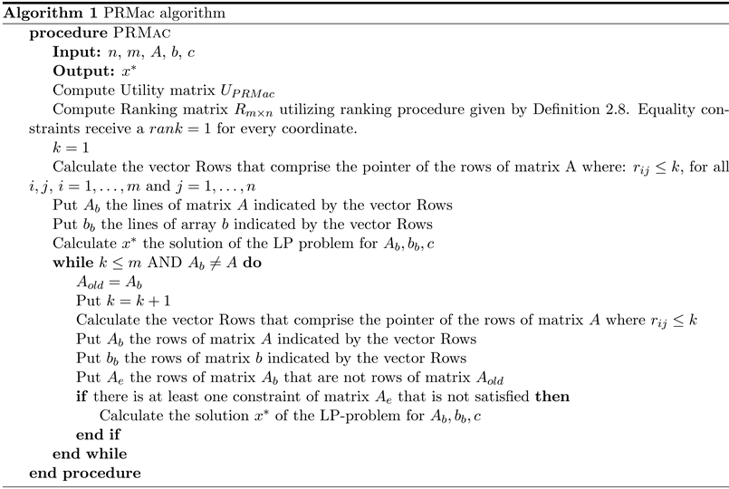
3.5. The Proximity Ranking Matrix (PRMac) Algorithm

In the first of the two proposed algorithms, named Proximity Ranking Matrix (PRMac), the Utility matrix given in Definition 11 is used. Specifically, the presented algorithm takes under consideration for each constraint the proximity of $a_{ij}$ to the corresponding $c_j$ , for $j=\mathrm{1,}\cdots \mathrm{,}n$ . The rising ranking indicates the possibility each constraint has to be binding. The constraints with smaller rankings are assumed to the more likely to be the binding ones. Especially for the equality constraints, since they are classified to be binding in advance, they should receive a $rank=1$ for every coordinate. In the proposed algorithm, the step-by-step procedure presented in [9] is utilized and the constraints are inserted by groups according to their ranking.

Specifically, the proposed algorithm gradually puts into classes the constraints of the LP problem, in order to solve a smaller problem, by considering the ranking of each variable. For this scaled insertion, the order given by the ranking matrix is taken under consideration, thus the smaller rankings per each variable are prioritized. During this insertion, the constraints that have not been used are checked according to their ranking, whether they are satisfied or not. In case they are satisfied, by making use of the Theorem 3.1 presented in [14] , the solution that has been found is not affected. In the opposite case, they must be added to the existing system and a new solution point is searched. Thus, progressive insertion of the useful constraints for solving the given LP problem is taking place, by classifying the constraints according to the possibility to be binding. As the process evolves, the majority of the remaining constraints are utilized for the verification of an optimal solution. As a result, the minority of the remaining constraints is expected to be used in the solving procedure of the given LP problem.

The proposed algorithm PRMac, is presented in Algorithm 1.

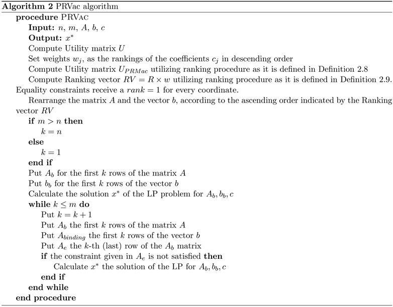
3.6. The Proximity Ranking Vector (PRVac) Algorithm

A different approach is the information that arises from each line of the utility matrix by making use of the PRMac algorithm, to be substituted from a number. Thus, the matrix is substituted from a vector. In order to accomplish this, techniques that calculate the norms of the vectors can be used, for instance $L_1\mathrm{,}{L}_2\mathrm{,}\cdots \mathrm{,}{L}_{\infty }$ or statistical indicators like mean, median, geometric mean, harmonic mean, etc. By making use of the same information as in the PRMac algorithm, the new proposed algorithm, named Proximity Ranking Vector (PRVac) transforms the Utility matrix $U_{PRMac}$ to a proximity vector, by applying $L_1$ norm for each row of the Utility matrix. The elements of the proximity vector are derived from the inner product of the vector’s ranking of coefficients $c_j$ of the objective function with the vector of the rankings $u_{ij}$ , where $u_{ij}$ is given by Definition 12 for the i-th constraint. As a result, a ranking vector as it is given in Definition 13 is derived.

On the contrary, with the proposed PRMac algorithm, the priority of the constraints is given in vector form instead of a matrix. Thus, the progressive insertion of the constraints is implemented by ascending priority order instead of priority groups, using the Theorem 3.1 presented in [14] , as before.

The proposed PRVac algorithm is presented in Algorithm 2. A simple example of the PRMac and PRVac algorithms is given in the next section.

4. Numerical Example

$\begin{array}{l}\text{Maximize}z=c^{\text{T}}x\\ \text{subject}\text{to}Ax\le b\\ x\ge 0\end{array}$ , where: $A=\left(\begin{array}{cc}1& 2/7\\ 3/7& 5/7\\ 1& 6/7\\ 1/7& 1/7\\ 3/7& 4/7\end{array}\right)$ , $b=\left(\begin{array}{c}2\\ 15/7\\ 6\\ 1\\ 12/7\end{array}\right)$ , $c=\left(\begin{array}{c}4/7\\ 3/7\end{array}\right)$ .

The optimum point is $x^{*}=\left(\begin{array}{c}1.455\\ 1.909\end{array}\right)$ and the binding constraints are the 1^st and the 5^th ones.

Compute Utility matrix by relation (2) and the corresponding ranking matrix

$U_{PRMac}=\left(\begin{array}{rr}\hfill 3/7& \hfill 1/7\\ \hfill 1/7& \hfill 2/7\\ \hfill 3/7& \hfill 3/7\\ \hfill 3/7& \hfill 2/7\\ \hfill 1/7& \hfill 1/7\end{array}\right),R=\left(\begin{array}{rr}\hfill 4& \hfill 1.5\\ \hfill 1.5& \hfill 3.5\\ \hfill 4& \hfill 5\\ \hfill 4& \hfill 3.5\\ \hfill 1.5& \hfill 1.5\end{array}\right)$ (4)

Set k = 1

For k = 1 no constraint is selected, so the system has a solution that tends to infinity.

Set k = 2

For k = 2, based on the ranking matrix R, Equation (4), three constraints are selected: the 1st, the 2nd and the 5th. Thus

$A=\left(\begin{array}{cc}1& 2/7\\ 3/7& 5/7\\ 3/7& 4/7\end{array}\right),b=\left(\begin{array}{c}2\\ 15/7\\ 12/7\end{array}\right)$ .

The optimum of the above problem satisfies the rest of the constraints of the given problem. Thus, in the following steps ( $k=3,4,5$ ) the PRMac algorithm checks, without solving the problem, that the rest of the constraints are met.

In Figure 1 two steps of the PRMac algorithm are depicted. In the left hand

Figure 1. Graphical representation of the algorithms PRMac and PRVac.

side, for $k=2$ where the first insertion of constraints takes place and in the right hand side the final step of the algorithm, with all the constraints included.

PRMac algorithm verifies that for $k=3,4,5$ the constraints given by the lines ${\epsilon }_3$ and ${\epsilon }_4$ are satisfied in the minimum point B defined for $k=2$ .

By utilizing PRVac algorithm after the computation of Utility matrix, weights are given as follows:

$w^{\text{T}}=(\; 1,2\; )$

$R=\left(\begin{array}{c}1\times 4+2\times 1.5\\ 1\times 1.5+2\times 3.5\\ 1\times 4+2\times 5\\ 1\times 4+2\times 3.5\\ 1\times 1.5+2\times 1.5\end{array}\right)=\left(\begin{array}{c}7\\ 8.5\\ 14\\ 11\\ 4.5\end{array}\right)$ (5)

The PRVac algorithm, in its first step for $k=n=2$ , inserts the fifth and the first constraints that are the binding constraints of the problem. Thus, it will give the point B as the optimum for the given LP-problem.

On the left-hand side of Figure 2, the ranking of the proximity of the constraints by coordinate is depicted according to the matrix R of the relation (4) for the PRMac algorithm. The corresponding representation for the matrix R, as given in relation (5), of the PRVac algorithm is given on the right-hand side of Figure 2. Because of the fact that the PRVac algorithm makes an overall consideration of the rankings, due to uniformity, the rankings have been represented in the bisector of the first quadrant. In both figures, the numbering of the ranking vectors corresponds to the numbering of the constraints. The second constraint, in black, is chosen by the PRMac algorithm because it has the same ranking as

Figure 2. Graphical representation of prioritization zones made by proximity rankings using R matrices of the PRMac and the PRVac algorithms.

the fifth constraint, in red, in terms of the first coordinate. The binding constraints, the first and fifth ones, are shown in red. With the PRVac algorithm, the second constraint is ranked to be third. Note that the optimal point has been located already by using the first and the fifth constraints, which have been chosen as those with the smallest ranking.

5. Numerical Results

The R package was used for the numerical results [36] - [41] . The multivariate analysis was performed using mgcv and nlme libraries [42] - [48] . Graphs have been made using the libraries ggplot2, gridExtra, RColorBrewer and sjplot [49] - [55] while for the formatting of the tables libraries htmltools, kableExtra and jtools have been used [56] [57] [58] . Moreover, hierarchical regression trees were implemented using rpart and rpart.plot R-libraries [59] [60] . The data files are all deposited to Github and it is possible to grant access to whoever it is desired to do so through the link given in [61] .

From all those mentioned above, it can be noticed that the PRVac algorithm makes gradual insertion of the constraints in the LP problem that is going to be solved, contrary to the PRMac algorithm where the insertion takes place in groups (their number tends to the dimension n of the LP problem) and the number is analogous to the dimension of the LP problem, so it increases together with the increment of the dimension. Thus, the PRMac algorithm inserts large groups of constraints regardless they are binding or not, whilst the PRVac algorithm inserts a constraint only after checking it for being binding. As a result, while the dimension of the problem increases, this feature gives the PRVac an advantage over the PRMac algorithm, whereas in LP problems with a few number of constraints, the PRMac has an advantage, because of the insertion of small groups of constraints. For the testing of the proposed algorithms were used:

• Set of 69 well-known benchmarks (netlib problems) [11] [12] , where the number of the variables is significantly bigger than the number of the constraints (subsection 5.1).

• Random problems, where the number of the constraints is significantly bigger than the number of the variables (subsection 5.2).

5.1. Random LP-Problems

5.1.1. Creating the Random LP-Problems

The random LP-problems are constructed by randomly selected variables and coefficients as follows:

• Dimension of each LP problem $n\in \left[\mathrm{3,100}\right]$ , $n\in N$ ,

• Number of constraints $m\in \left[10\cdot n\mathrm{,15}\cdot n\right]$ , $m\in N$ ,

• $a_{ij}\in \left[-\mathrm{1,1}\right]$ ,

• $c_j\in \left[-\mathrm{1,1}\right]$ .

In order to increase the probability that a solution exists in the randomly constructed LP-problems, a random solution ( $x^{\mathrm{<mo>\; *\; </mo>}}$ ) of the created LP-problem under the assumption the coefficients of $x^{\mathrm{<mo>\; *\; </mo>}}$ to be randomly chosen in the interval $\left[\mathrm{0,1}\right]$ is given. Afterwards, $b=a_{ij}\cdot x^{\mathrm{<mo>\; *\; </mo>}}$ is calculated and perturbation, with random noise of scale 10% takes place. The chosen perturbation is not particularly great, because the objective is the creation of random LP problems that can be solved and it is a common assumption that while the dimension of the LP problem n increases, bigger perturbation in b could make extremely difficult the existence of an LP problem that can be solved.

Figure 3 and Figure 4 depicts the histogram of the number of variables and

Figure 3. Histogram of number of variables where different colors indicate the number of binding constraints (n.binding).

Figure 4. Histogram of number of constraints where different colors indicate the number of binding constraints.

constraints for the test problems accordingly. Furthermore, Figure 5 shows the histogram of the percentages of binding constraints in the total number of constraints. In all those figures, a colourful escalation has been applied, depending on the number of binding constraints of the LP problem.

Table 1 represents the frequencies of the ratio of the number of binding constraints divided by the total number of constraints. As can be observed, the greater frequency 3499 lies in the interval $\left(\mathrm{0.12,0.14}\right]$ followed by the frequency 2748 in the interval $\left(\mathrm{0.14,0.16}\right]$ . Note that, the average of the binding constraints is 13.168% of a total number of constraints.

Figure 5. Histogram of percentage of the binding constraints.

Table 1. Frequency table of the ratio of the number of binding constraints divided by the total number of constraints.

Remark 1. The constraints that satisfy the relation $\left|b-A\cdot x^{\mathrm{<mo>\; *\; </mo>}}\right|\le {10}^{-12}$ are considered to be the binding ones. Without further checking the linear independence of these constraints, this relationship does not ensure that the constraints are binding and not weakly redundant. Therefore, in numerical results, there is a possibility that a number of weakly redundant constraints may be included in the binding constraints.

5.1.2. Including Binding Constraints by a Proper Ranking

As has already been mentioned, whenever a mathematical formulation is given in order to describe a real-world LP problem, usually the number of constraints is more than the necessary ones [2] . Furthermore, when dealing with real-world LP problems, it is impossible to know which and how many the binding constraints are before spotting an optimal solution in case it exists. Utilizing the first k ranked constraints per variable the prop.binding is defined as:

$\text{prop}\text{.binding}=\frac{\text{Numberofbindingconstraintsselectedusing}k}{\text{Totalnumberofbindingconstraints}}$

An ascending ranking procedure for classifying the constraints is considered to be successful if small rankings are given to the binding constraints where the number k, $1<k<m$ , is randomly selected. In order to examine whether the constraints having small ranking in the PRMac and PRVac algorithms have a greater probability to be bindings, hierarchical regression trees for prop.binding are utilized. Specifically, hierarchical regression trees were used to check if the size of k (hence k/m) affects the size of the prop.binding. Figure 6 presents the hierarchical regression tree for prop.binding using the PRMac algorithm where $\text{k}\text{.over}\text{.m}=\frac{k}{m}$ is the independent variable. Note that in every node or leaf of the hierarchical tree, it has depicted the percentage of the sample that the node or the leaf corresponds to, as well as the mean value of the dependent variable

Figure 6. Hierarchical regression tree for PRMac algorithm. The gradations of colors from red to green reflect the average from the lowest to the highest average values of prop.binding.

(prob.binding). The leaves of the tree, refer to the conditions of the independent variable. When the condition is satisfied, then the left-hand side leaf of the hierarchical tree is followed, otherwise, the right-hand side leaf is followed. Moreover, in order to reduce the risk of over-fitting, the process of pruning has been applied. From Figure 6, the following conclusions can be extracted:

• On average the prop.binding for the 10,000 randomly constructed LP-problems is 0.97 (root of the tree).

• If k is selected such that k/m is greater than 0.12 (that happens in 89% of the random LP problems) the number of prop.binding is 0.99, which means that the 99% of the binding constraints has been selected (the rightmost leaf of the tree).

• If k is selected such that k/m is greater than 0.037 (that happens in 97% of the random LP-problems) the number of prop.binding is 0.98, which means that the 98% of the binding constraints has been selected (the node over the rightmost leaf of the tree).

Thus, the PRMac algorithm is able to achieve high percentage in locating the bindings in a small number of selected constraints per variable, which leads to the conclusion that the information from every variable is important.

Figure 7 represents the hierarchical regression tree for the PRVac algorithm. At this point, it is worthy to notice that the PRVac algorithm summarizes the information of the ranking matrix (which is used in PRMac algorithm) into a vector. A random number of k selected constraints, $1<k<m$ , is defined and the first k ranked constraints are used.

• On average the prop.binding for the 10,000 randomly constructed LP problems is 0.58 (root of the tree).

• If k is selected such that k/m is greater than 0.75 (that happens in 27% of the random LP problems of the sample) the number of prop.binding is 0.91, which means that the 91% of the binding constraints has been selected (the rightmost leaf of the tree).

Figure 7. Hierarchical regression tree for PRVac algorithm. The gradations of colors from red to green reflect the average from the lowest to the highest average values of prop.binding.

• If k is selected such that k/m is greater than 0.52 (that happens in 52% of the random LP problems of the sample) the number of prop.binding is 0.8, which means that the 80% of the binding constraints has been selected (the node over the rightmost leaf of the tree).

5.1.3. Relation of the prop.binding with the Ranking

In this subsection the research is focused on the model which would be able to interpret better the value of the prob.binding in relation to the ratio $\frac{k}{m}$ , by making use of the results from the randomly created LP-problems.

In Figure 8, the scatter plot of the number of variables with the number of constraints for the 10,000 randomly constructed LP-problems is presented. In the same figure, for every LP problem, the ratio of detecting binding constraints has been illustrated colourfully by making use of darker colours for the smaller ratio and lighter colours for the bigger values. This specific illustration has been selected in order to detect visually whether the PRMac algorithm is behaving in the same way for all LP-problems having m constraints and n dimensions. This illustration reveals on the one hand that yellow dots correspond to a high percentage for the prob.binding are the dominant ones—as a result the binding constraints are gathered in low rankings independently of the value of the ratio $\frac{k}{m}$ —and on the other hand the darker dots correspond in low percentage for the prob.binding,have a rather rare appearance and are evenly distributed among the yellow dots.

Figure 9(a) presents on the left-hand side the scatter plot of the prob.binding in relation with the ratio $\frac{k}{m}$ and Figure 9(b) presents the same figure with the

Figure 8. Number of variables and number of constraints of the 10,000 random LP-problems.

(a)(b)

Figure 9. Scatter plots of the prop.binding variable in accordance with (a) k/m (b) log(k/m).

logarithmic transformation of the x axis. The left hand side of the scatter plot confirms the fact that for small values of the ratio $\frac{k}{m}$ , small changes of it cause big increment in prop.binding. While the value of the ratio $\frac{k}{m}$ increases, the rate of change decreases. This exponential behaviour of the function leads to the logarithmic transformation of the ratio $\frac{k}{m}$ . Thus, on the right-hand side of Figure 9(b), a sigmoid relation that connects the possibility of including in the first k constraints the bindings and the logarithm of the ratio $\frac{k}{m}$ is appeared.

ANOVA Table 2 shows that the dependent variable prob.binding is affected by the ratio $\frac{k}{m}$ .

The influence of k/m on prop.binding is confirmed by ANOVA table given in Table 2. Hence, the logit model of the log of k over m is applied and the result of this model is presented in Table 3.

From Table 3 it is confirmed that $\log \left(\frac{k}{m}\right)$ is statistically significant (p-value < 0.001). Moreover, the coefficient of $\frac{k}{m}$ (41.40) derives that the increment of $\frac{k}{m}$ will result in a fast increment of the ratio for the detection of the binding constraints.

Figure 10 presents the graph of the logistic function (black curve) derived from the logit model. It can be observed that the points corresponding to the random problems are gathered by the majority above the approximation curve, so the approximated value underestimates the performance of the algorithm. As a result, in the randomly generated LP problems, the usage of $\frac{k}{m}$ of the constraints is expected to be better in the detection of the binding constraints than the approximation.

5.2. NETLIB LP-Problems

The proposed algorithms were applied to the well-known 69 benchmark problems (netlib problems) [11] [12] .

In Table 4 the results from the netlib problems are depicted with the following labels:

• netlib is the name of the netlib problem.

• n the dimension of each LP problem.

• m the number of constraints.

• n.binding the percentage of the number of the constraints that are binding or weakly redundant constraints (see Remark in subsection 5.2).

• 50 is the number of constraints that must be chosen after ranking the constraints with the proper algorithm, in order to include 50% of the n.binding constraints of the LP problem.

Table 2. ANOVA Table of the prop.binding in relation with k over m.

Table 3. Logit model.

Figure 10. The graph of the logistic function derived from the logit model.

Table 4. Ranking results of the constraints by making use of the PRMac, PRVac, RAD and GRAD algorithms in netlib problems.

• 90 is the number of the constraints that must be chosen after ranking the constraints with the proper algorithm, in order to include 90% of the n.binding constraints of the LP problem.

• Sparsity the percentage of matrix A (or vectors b and c) elements that are non-zero.

From Table 4 it can be derived that one feature of the netlib problems is that the number of binding constraints is significantly large (on average 78% of the constraints). It is worthy to mention, that those problems have a big percentage of coefficients equal to zero, both for the constraints and for the objective function. Specifically, on average 98.5% of the elements of array A are equal to zero (a sparsity of 0.015), 60.8% of elements of array b (a sparsity of 0.392) and 58.2% of elements of array c (a sparsity of 0.418) are equal to zero. Moreover, it is remarkable the fact that by making use of the PRMac algorithm. The constraints are ranked in such a way that the first 61% of them, including 90% of the binding constraints of the LP problem, considering the fact that the PRMac is implemented in problems with a large number of binding constraints.

From Table 4 it can be revealed that one feature of the netlib problems is that the number of the constraints is on average 1/3 of the number of the variables (941 constraints - 3587 variables).

In the random LP problems, the ranking of the constraints takes place in such a way that for solving the LP problem, 90% of the constraints are used on average. For the netlib problems, it can be observed that the first group of the constraints for the PRMac algorithm can include 61% of the constraints.

Moreover, from Table 4 it can be observed that the average for including in the first k constraints the 50% of the binding constraints is slightly better in the PRVac algorithm, 0.48 instead of 0.55. For 90% of the constraints, the situation is reversed clearly in favour of the PRMac algorithm (0.61 instead of 0.87). On the other hand, the GRAD algorithm is proved to be slightly better in comparison with RAD, for both those cases, with the corresponding values to be 0.56 instead of 0.58 and 0.82 instead of 0.86. Overall PRVac is proved to be slightly better in 50% of the binding constraints, while for 90% of the constraints, PRMac is proved to be far a way better than all the others.

There are Netlib problems where due to their “nature” (the same $a_{ij}$ for one variable in all the constraints) the PRMac algorithm gives “poor” classification in some variables of the constraints. Thus, the PRMac algorithm attributes to a large number of the constraints the same ranking number. On the contrary, by making use of the PRVac algorithm this disadvantage is overcome and the Netlib problems can be faced efficiently. Consequently, in general, it is preferable when matrix A creates a “poor” classification, to make use of the PRVac algorithm.

5.3. An Overview of the Numerical Results of PRMac and PRVac Algorithm

In order to calculate the mean number of iterations while solving an n-dimensional LP problem with m constraints by using the Simplex Method [62] [63] [64] [65] presented the following approximation relations:

$T_{L_1}=0.486{\left(m+n\right)}^{1.12}\mathrm{,}{T}_{L_2}=0.546{\left(m+n\right)}^{1.05}$ (6)

where L₁ and L₂ are the minimization norms used in the regression process. As it can be observed, because the exponent in $T_{L_2}$ is smaller in comparison with $T_{L_1}$ , $T_{L_2}$ is expected to do a smaller number of iterations. Moreover, for the same problem by using the dual Simplex method in [62] [63] [64] [65] , the following relation is given for both of the norms:

$T=0.8\min {\left(m\mathrm{,}n\right)}^{1.46}$ (7)

The above relations calculate the mean number of iterations. As in every iteration, the dimension of the utilized vectors is m + n and every reduction in the number of m leads both in the reduction of the mean number of iterations as well as of the dimension of vectors used in every iteration.

Next, the relations (6) and (7) are going to be used in order to evaluate the reduction of the computational cost given under the proposed algorithms, for the netlib problems provided in Table 4. Based on the percentages derived from columns Mac90 and Vac90 of Table 4, it is estimated that the percentage of the constraints required in order to include the 100% of the binding constraints lie in the half distance between the 100% and Mac90 or the 100% and Vac90 accordingly. It gives a percentage of 79.19 for the PRMac algorithm and 93.07 for the PRVac algorithm, respectively.

According to relation (6), if the Simplex method is going to be used in order to solve the given LP problem, the mean number of iterations is going to be approximately 501 - 703, and the dimension of vectors used in every iteration is approximately 663, because $T_{L_1}=501$ and $T_{L_2}=703$ .

So, by making use of the PRMac algorithm, the reduction of m by 20.81 leads on average in 101 - 150 fewer iterations, while the vectors used in every iteration have on average 177 fewer dimensions. This is equivalent to a reduction of the iterations from 5.54% to 10.34% with the PRMac algorithm. Likewise, by making use of the PRVac algorithm, a reduction of m by 6.93% leads on average in 34 - 50 fewer iterations, while the vectors used in every iteration, have on average 92 fewer dimensions. This is equivalent to a reduction of the iterations from 6.94% to 8.72% with the PRVac algorithm.

Similar results derive from (7) concerning the Dual Simplex method. The usage of the Dual Simplex method requires approximately 238 iterations and the vectors used in every iteration have on average 663 dimensions. By making use of the PRMac algorithm, the number of vectors used in every iteration, have on average 177 fewer coordinates. In case the dual simplex method is used, the reduction of the iterations is going to be on average 5969, which leads to a percentage decrease of 63.01%. Whereas with the PRVac algorithm, the dimension of vectors used in every iteration has on average 92 fewer dimensions. In case the dual simplex method is used, the reduction of the iterations is going to be on average 2763, which leads to a percentage decrease of 40.27%. Despite the exceptional approach in ranking the binding constraints that become feasible by using $a_{ij}\ast c_j/b_i$ , the fact that primarily $b_i$ may be zero and secondarily if $c_j=0$ the j-th variable is not taken under consideration in the ranking of the constraints is a shortcoming. On the contrary, the proposed algorithms of this paper make use of proximity in the classification of the constraints, so both the coefficients of the constraints $a_{ij}$ as well as the coefficients of the objective function $c_j$ are taken into consideration, without worsening the functional cost. As a result, arithmetic operations between vectors do not take place and the precision of the operations is not affected. More precisely, in the PRVac algorithm, the classification takes place by taking into account the rankings per coordinate and by setting as weights the values of $c_j$ , giving the smaller value to the coordinate of $c_j$ having the greater absolute value. Netlib problems, have $b_i=0$ in a regular basis, so in order to test the RAD algorithm, $b_i$ was set to be $b_i={10}^{-64}$ instead of $b_i=0$ . In the same algorithm, the constraints are classified by considering as best the one with the biggest RAD (smallest ranking).

6. Conclusions and Further Research

In the present paper, two new algorithms for solving LP problems are presented. The proposed algorithms rank the constraints according to the possibility of being binding based on the idea of proximity which can be used in LP problems with a very large number of constraints. Moreover, in the theoretical framework of the proposed algorithms already known algorithms can be involved. By making use of the distance of the coefficients of the constraints with the corresponding coefficients of the objective function, the proposed PRMac and PRVac algorithms, utilize a utility matrix or a utility vector correspondingly. In order to rank the constraints the process is simple, as it is only based on comparisons between the coefficients and does not require any further calculations.

For testing PRMac and PRVac algorithms, a generator of random LP problems is addressed for constructing 10,000 random LP problems of dimension n with m constraints, where $m\gg n$ . As has already been mentioned a generator of random linear problems with many constraints may represent a wide range of real-world problems. From the numerical results, it is derived that in the majority of the random LP problems, the proposed algorithms are considered to be efficient since they rank the constraints in such a way that the binding ones are gathered in a lower ranking. Moreover, the application of the proposed algorithms to problems of the Netlib repository gave slightly better numerical results than their application to random problems. The algorithms that use as a classification criterion a ratio where $c_j$ lies in the numerator, multiply the numerator with zero, even when a single $c_j=0$ . Thus, the other variable of the numerator does not affect the result. In reality, though, $c_j$ affects only the constraints but not the objective function. For instance, the constraints that may be met in transportation companies (logistics), may affect the profits but are not related to the company. As a result, the company has not the ability to improve the constraints in order to increase its profits. In the objective function that reflects the profits, these variables exist with a $c_j=0$ coefficient. In the methods where $c_j$ lies in the numerator, it remains unchanged, whether the aforementioned variables exist or not, while it is well known that they contribute significantly in the definition of the feasible area. With the proposed methodology in this paper, the proximity of each $a_{ij}$ with the corresponding $c_j$ is calculated, so even if $c_j=0$ , the j-th variable is taken into account for the ranking and the classification of the constraints. The already existing algorithms use a measure of comparison and afterwards based on this measure. They rank the constraints. The renovation of the proposed algorithms here is that by knowing in advance that they are intended in ranking instead of using precise data. They focus in advance on ranking the proximity of $a_{ij}$ with the corresponding $c_j$ and based on those values they classify the constraints. In other words, the achievement of great precision in the arithmetic operations is sacrificed, just in order for the algorithms to remain efficient under any circumstances as it was shown above. In general, when dealing with optimization problems with constraints, the constraints contribute the major part in comparison with the objective function, because they define the feasible area of the LP problem. As it concerns the objective function, the only point of interest is the extreme point that lies in the feasible area. So, it is obvious that an efficient algorithm should prioritize the constraints over the objective function.

As a future research, extensive use of the proposed theoretical framework can be done, by making use of different utility functions or by combining different techniques. The promising results of the present paper reveal the worthiness of dedicating time and research for the adaptation of the proposed algorithms in various categories of LP problems with constraints.

Moreover, it is worth to study the implementation of the substitution of the utility matrix used in the PRMac algorithm by utilizing a different norm or different statistical indices of univariate analysis.

Acknowledgements

The authors wish to acknowledge Prof. Theodoula N. Grapsa for her helpful suggestions.

Conflicts of Interest

The authors declare no conflicts of interest regarding the publication of this paper.

References

[1]	Bertsimas, D. and Tsitsiklis, J.N. (1997) Introduction to Linear Optimization. Athena Scientific, Belmont. http://athenasc.com/linoptbook.html
[2]	Sumathi, P., Balachander, P., Karpagam, A. and Pugazhenthi, P. (2015) A New Tactic for Finding Irrelevant Constraints in Linear Programming Problems. International Journal of Scientific & Engineering Research, 6, 66-69.
[3]	Tsarmpopoulos, D.G., Nikolakakou, C.D. and Androulakis, G.S. (2020) The Sign of the Slope of the Objective Function on Identifying Binding Constraints in LP Problems. 24th Panhellenic Conference on Informatics (PCI 2020), Athens, 20-22 November 2020, 260-263. https://doi.org/10.1145/3437120.3437320
[4]	Corley Jr., H.W. and Rosenberger, J.M. (2011) System, Method and Apparatus for Allocating Resources by Constraint Selection. https://patentimages.storage.googleapis.com/28/74/03/78654f1a05591b/US8082549.pdf
[5]	Corley, H.W., Noroziroshan, A. and Rosenberger, J.M. (2017) Posterior Constraint Selection for Nonnegative Linear Programming. American Journal of Operations Research, 7, 26-40. https://doi.org/10.4236/ajor.2017.71002
[6]	Noroziroshan, A., Corley, H.W. and Rosenberger, J.M. (2015) A Dynamic Active-Set Method for Linear Programming. American Journal of Operations Research, 5, 526-535. https://doi.org/10.4236/ajor.2015.56041
[7]	Saito, G. (2012) Constraint Optimal Selection Techniques (Costs) for Linear Programming. https://rc.library.uta.edu/uta-ir/handle/10106/11066
[8]	Saito, G., Corley, H.W., Rosenberger, J.M., Sung, T.-K. and Noroziroshan, A. (2015) Constraint Optimal Selection Techniques (Costs) for Nonnegative Linear Programming Problems. Applied Mathematics and Computation, 251, 586-598. https://doi.org/10.1016/j.amc.2014.11.080
[9]	Sumathi, P. (2016) A New Approach to Solve Linear Programming Problem with Intercept Values. Journal of Information and Optimization Sciences, 37, 495-510. https://doi.org/10.1080/02522667.2014.996031
[10]	Corley, H.W., Rosenberger, J., Yeh, W.-C. and Sung, T.K. (2006) The Cosine Simplex Algorithm. The International Journal of Advanced Manufacturing Technology, 27, 1047-1050. https://doi.org/10.1007/s00170-004-2278-1
[11]	Browne, S., Dongarra, J., Grosse, E. and Rowan, T. (1995) The Netlib Mathematical Software Repository. D-Lib Magazine, 1, 96. https://doi.org/10.1045/september95-browne
[12]	Dongarra, J. and Grosse, E. (1985) Netlib Repository at UTK and ORNL. http://www.netlib.org/
[13]	Telgen, J. (1983) Identifying Redundant Constraints and Implicit Equalities in Systems of Linear Constraints. Management Science, 29, 1209-1222. https://doi.org/10.1287/mnsc.29.10.1209
[14]	Caron, R.J., McDonald, J.F. and Ponic, C.M. (1989) A Degenerate Extreme Point Strategy for the Classification of Linear Constraints as Redundant or Necessary. Journal of Optimization Theory and Applications, 62, 225-237. https://doi.org/10.1007/BF00941055
[15]	Gal, T. (1992) Weakly Redundant Constraints and Their Impact on Postoptimal Analyses in LP. European Journal of Operational Research, 60, 315-326. https://doi.org/10.1016/0377-2217(92)90083-L
[16]	Stojkovic, N.V. and Stanimirović, P.S. (2001) Two Direct Methods in Linear Programming. European Journal of Operational Research, 131, 417-439. https://doi.org/10.1016/S0377-2217(00)00083-7
[17]	Estiningsih, Y. and Tjahjana, R.H. (2019) Modified Stojkovic-Stanimirovic Method to Find Redundant Constrains in Linear Programming Problems. Journal of Physics: Conference Series, 1321, Article ID: 022074. https://doi.org/10.1088/1742-6596/1321/2/022074
[18]	Sumathi, P. and Gangadharan, A. (2014) Selection of Constraints with a New Approach in Linear Programming Problems. Applied Mathematical Sciences, 8, 1311-1321. https://doi.org/10.12988/ams.2014.42121
[19]	Yang, Y.G. (2021) A Modified Row Pivot Simplex Algorithm. https://arxiv.org/abs/2107.08468v1
[20]	Brearley, A.L., Mitra, G. and Williams, H.P. (1975) Analysis of Mathematical Programming Problems Prior to Applying the Simplex Algorithm. Mathematical Programming, 8, 54-83. https://doi.org/10.1007/BF01580428
[21]	Ioslovich, I. and Gutman, P.-O. (2000) Robust Redundancy Determination and Evaluation of the Dual Variables of Linear Programming Problems in the Presence of Uncertainty. IFAC Proceedings Volumes, 33, 149-154. https://doi.org/10.1016/S1474-6670(17)36220-1
[22]	Ioslovich, I. (2001) Robust Reduction of a Class of Large-Scale Linear Programs. SIAM Journal on Optimization, 12, 262-282. https://doi.org/10.1137/S1052623497325454
[23]	Sumathi, P. and Paulraj, S. (2013) Identification of Redundant Constraints in Large Scale Linear Programming Problems with Minimal Computational Effort. Applied Mathematical Sciences, 7, 3963-3974. https://doi.org/10.12988/ams.2013.36325
[24]	Llewellyn, R.W. (1964) Linear Programming. Holt, Rinehart and Winston, New York. http://lib.ugent.be/catalog/rug01:000485171
[25]	Telgen, J. (1979) OnR.W. Llewellyn’s Rules to Identify Redundant Constraints: A Detailed Critique and Some Generalizations. Zeitschrift für Operations Research, 23, 197-206. https://doi.org/10.1007/BF01919484
[26]	Paulraj, S., Chellappan, C. and Natesan, T.R. (2006) A Heuristic Approach for Identification of Redundant Constraints in Linear Programming Models. International Journal of Computer Mathematics, 83, 675-683. https://doi.org/10.1080/00207160601014148
[27]	Veni, K.K. and Balachandar, S.R. (2010) A New Heuristic Approach for Large Size Zero One Multi Knapsack Problem Using Intercept Matrix. International Journal of Computing Science and Mathematics, 4, 259-263.
[28]	Estiningsih, Y., Farikhin and Tjahjana, R.H. (2018) A Comparison of Heuristic Method and Llewellyn’s Rules for Identification of Redundant Constraints. Journal of Physics: Conference Series, 983, Article ID: 012069. https://doi.org/10.1088/1742-6596/983/1/012083
[29]	Estiningsih, Y., Farikhin and Tjahjana, R.H. (2019) Some Methods for Identifying Redundant Constraints in Linear Programming. Journal of Physics: Conference Series, 1321, Article ID: 022074. https://doi.org/10.1088/1742-6596/1321/2/022074
[30]	Nikolopoulou, E.I., Manoussakis, G.E. and Androulakis, G.S. (2019) Locating Binding Constraints in LP Problems. American Journal of Operations Research, 9, 59-78. https://doi.org/10.4236/ajor.2019.92004
[31]	Tsarmpopoulos, D.G., Nikolakakou, C.D. and Androulakis, G.S. (2021) Solving LP Problems Using the Ranking of the Ratio of Constraints’ Coefficients. Proceedings of the 25th Pan-Hellenic Conference on Informatics, PCI’21, Volos, 26-28 November 2021, 130-133. https://doi.org/10.1145/3503823.3503848
[32]	Tsarmpopoulos, D.G., Nikolopoulou, E.I., Nikolakakou, C.D. and Androulakis, G.S. (2022) A Combination of a Proximity Technique and Weighted Average for LP Problems. In: Proceedings of the 26th Pan-Hellenic Conference on Informatics, PCI’22, Athens, 25-27 November 2022, 181-186. https://doi.org/10.1145/3575879.3575990
[33]	Hillier, F.S. and Lieberman, G.J. (2015) Introduction to Operations Research. 10th Edition, McGraw-Hill, New York.
[34]	Paulraj, S. and Sumathi, P. (2010) A Comparative Study of Redundant Constraints Identification Methods in Linear Programming Problems. Mathematical Problems in Engineering, 2010, Article ID: 723402. https://doi.org/10.1155/2010/723402
[35]	Jibrin, S. and Stover, D. (2007) Identifying Redundant Linear Constraints in Systems of Linear Matrix Inequality Constraints. Journal of Interdisciplinary Mathematics, 10, 601-617. https://doi.org/10.1080/09720502.2007.10700521
[36]	The R Project for Statistical Computing. https://www.r-project.org/
[37]	Wickham, H., Hester, J. and Bryan, J. (2022) readr: Read Rectangular Text Data. https://readr.tidyverse.org https://github.com/tidyverse/readr
[38]	Xie, Y.H. (2016) Bookdown: Authoring Books and Technical Documents with R Markdown. Chapman and Hall/CRC, Boca Raton. https://doi.org/10.1201/9781315204963
[39]	Xie, Y.H. (2022) Bookdown: Authoring Books and Technical Documents with R Markdown. R Package Version 0.25. https://bookdown.org/yihui/bookdown
[40]	Wickham, H., François, R., Henry, L., Müller, K. and Vaughan, D. (2023) dplyr: A Grammar of Data Manipulation. https://dplyr.tidyverse.org https://github.com/tidyverse/dplyr
[41]	Xie, Y.H. (2021) knitr: A General-Purpose Package for Dynamic Report Generation in R. R Package Version 1.37. https://yihui.org/knitr/
[42]	Wood, S. (2023) mgcv: Mixed GAM Computation Vehicle with Automatic Smoothness Estimation. R Package Version 1.9-0. https://CRAN.R-project.org/package=mgcv
[43]	Pinheiro, J., Bates, D. and R-Core (2021) nlme: Linear and Nonlinear Mixed Effects Models. R Package Version 3.1-153. https://svn.r-project.org/R-packages/trunk/nlme/
[44]	Wood, S.N. (2011) Fast Stable Restricted Maximum Likelihood and Marginal Likelihood Estimation of Semiparametric Generalized Linear Models. Journal of the Royal Statistical Society (B), 73, 3-36. https://doi.org/10.1111/j.1467-9868.2010.00749.x
[45]	Wood, S.N., Pya, N. and Safken, B. (2016) Smoothing Parameter and Model Selection for General Smooth Models (with Discussion). Journal of the American Statistical Association, 111, 1548-1575. https://doi.org/10.1080/01621459.2016.1180986
[46]	Wood, S.N. (2004) Stable and Efficient Multiple Smoothing Parameter Estimation for Generalized Additive Models. Journal of the American Statistical Association, 99, 673-686. https://doi.org/10.1198/016214504000000980
[47]	Wood, S.N. (2017) Generalized Additive Models: An Introduction with R. 2nd Edition, Chapman and Hall/CRC, Boca Raton. https://doi.org/10.1201/9781315370279
[48]	Wood, S.N. (2003) Thin-Plate Regression Splines. Journal of the Royal Statistical Society (B), 65, 95-114. https://doi.org/10.1111/1467-9868.00374
[49]	Wickham, H., Chang, W., Henry, L., Pedersen, T.L., Takahashi, K., Wilke, C., Woo, K., Yutani, H. and Dunnington, D. (2021) ggplot2: Create Elegant Data Visualisations Using the Grammar of Graphics. R Package Version 3.4.4. https://CRAN.R-project.org/package=ggplot2
[50]	Auguie, B. and Antonov, A. (2017) gridExtra: Miscellaneous Functions for “Grid” Graphics. R Package Version 2.3. https://CRAN.R-project.org/package=gridExtra
[51]	Neuwirth, E. (2014) RColorBrewer: ColorBrewer Palettes. R Package Version 1.1-3. https://CRAN.R-project.org/package=RColorBrewer
[52]	Lüdecke, D. (2021) sjPlot: Data Visualization for Statistics in Social Science. R Package Version 2.8.10. https://strengejacke.github.io/sjPlot/
[53]	Garnier, S., Ross, N., Rudis, R., Camargo, A.P., Sciaini, M., et al. (2021) viridis: Colorblind-Friendly Color Maps for R. R Package Version 0.6.4. https://CRAN.R-project.org/package=viridis
[54]	Garnier, S., Ross, N., Rudis, R., Camargo, A.P., Sciaini, M., et al. (2021) viridis: Colorblind-Friendly Color Maps for R. viridislite Package Version 0.4.2. https://CRAN.R-project.org/package=viridisLite
[55]	Wickham, H. (2016) ggplot2: Elegant Graphics for Data Analysis. Springer-Verlag, New York. https://doi.org/10.1007/978-3-319-24277-4_9
[56]	Cheng, J., Sievert, C., Schloerke, B., Chang, W., Xie, Y.H. and Allen, J. (2021) htmltools: Tools for HTML. R Package Version 0.5.2. https://github.com/rstudio/htmltools
[57]	Long, J.A. (2021) jtools: Analysis and Presentation of Social Scientific Data. R Package Version 2.1.4. https://jtools.jacob-long.com
[58]	Zhu, H., et al. (2021) kableExtra: Construct Complex Table with “kable” and Pipe Syntax. https://CRAN.R-project.org/package=kableExtra
[59]	Therneau, T., et al. (2023) rpart: Recursive Partitioning and Regression Trees. R Package Version 4.1.21. https://CRAN.R-project.org/package=rpart
[60]	Milborrow, S. (2021) rpart.plot: Plot rpart Models: An Enhanced Version of plot.rpart. R Package Version 3.1.1. https://cran.r-project.org/web/packages/rpart.plot/inde
[61]	Data Repository for PRMAc and PRVac Algorithm for Linear Programming. https://github.com/gandroul/PRMac-PRVac
[62]	Nering, E.D. and Tucker, A.W. (1992) Linear Programs & Related Problems: A Volume in the Computer Science and Scientific Computing Series. Elsevier, Amsterdam.
[63]	Maurer, S.B. (1994) Linear Programs and Related Problems, by Evar D. Nering and Albert W. Tucker. The American Mathematical Monthly, 101, 1022-1026. https://doi.org/10.1080/00029890.1994.12004586
[64]	Daniel, R.C. (1998) Review of Linear Programming: Foundations and Extensions by R.J. Vanderbei. The Journal of the Operational Research Society, 49, 94-94. https://doi.org/10.2307/3010658
[65]	Vanderbei, R.J. (2014) Linear Programming Foundations and Extensions. 4th Edition, Springer, New York. https://doi.org/10.1007/978-1-4614-7630-6