Derivation of a Formula for Mountain Height as a Function of Rank in Height

Edward J. Allen

Department of Mathematics and Statistics Texas Tech University, Lubbock, USA.

DOI: 10.4236/jamp.2023.1111225                

Abstract

The relationship between mountain height and rank in height for a mountainous region is examined. A stochastic differential equation model is derived for the evolution of mountain elevations. The derivation is based on simple assumptions about tectonic and erosion processes in mountain elevation dynamics. At any given time, the model yields a CIR-type probability density for mountain heights. As data are often available for mountains of greatest elevation in a region, the tail of the CIR density is studied and compared with mountain height data for the highest mountains in the region. The tail density is proportional to the product of a power of height and an exponential function of height, i.e., h^b-1exp(-ah) where h is mountain height and a and b are constants. The inverse distribution function of the tail probability density leads to a formula that relates rank in height to the corresponding mountain height. The formula provides, for example, a decreasing sequence of theoretical mountain heights for the region. The derived formula is tested against mountain height data sets for several mountainous regions in the British Isles, Continental Europe, Northern Africa, and North America. The derived formula provides an excellent fit to the mountain height data ranked by height.

Keywords

Mountain Height Distribution, SDE, Geophysics, Stochastic Model, Orology

1. Introduction

It has been hypothesized that mountains experience several phases including an initial growth phase caused by plate interactions and other tectonic events, a second stage where denudation processes and uplift interact against each other possibly at times balancing each other, and a final phase where mountain elevations gradually decline through erosion processes [1] . For example, it is estimated that, as the Alps erode at the top and regenerate from the earth’s mantle, the Alps lose and gain about a millimeter per year of elevation [2] . Rates of tectonic and denudation processes and the relative importance of tectonic versus climatic processes, erosion, and other denudation processes are currently undergoing much study and discussion [3] - [10] . In the present investigation, it is assumed that mountains are growing and declining through tectonic and denudation processes.

Mountain height distributions are of interest to geologists and naturalists as well as to mountaineering enthusiasts [2] [11] - [16] . As erosion and uplifting processes interact, some mountains disappear into the background as their heights decline below a certain level. However, data for the mountains of greatest elevation are thoroughly and accurately recorded with most of these mountains having unique identifying names. Through examination of the data available for the mountains of greatest elevation in a mountainous region, models of dynamic mountain growth and decline can be studied and compared.

In the present investigation, an Itô stochastic differential equation (SDE) model is derived for mountain elevation dynamics where it is assumed that the mountains are growing and declining through tectonic and climatic processes. The SDE model indicates that the mountain height distribution for long time after initial formation is approximately a type of Cox-Ingersoll-Ross (CIR) distribution. It is shown that the tail of the CIR distribution for the greatest mountain heights has the form $h^{b-1}\exp \left(-ah\right)$ where a and b are constants and h is mountain height. The inverse cumulative distribution function of the tail probability density leads to a specific function that relates rank in height to mountain height. The formula is tested against mountain height data sets for several mountain classifications in the British Isles, Continental Europe, Northern Africa, and North America, where thorough, well-documented data are available. The derived formula provides an excellent fit to mountain height data ranked by height.

Original contributions of the present investigation include the following.

· Based on a physical argument, a new formula is derived for mountain height as a function of rank in height for a mountainous region.

· The derivation follows from simple assumptions on tectonic and deundation processes in mountain elevation dynamics.

· The derived formula agrees very well with mountain height data of Europe, Africa, and North America.

In addition, for convenience, many of the mathematical symbols used in present investigation are tabulated and described in the Appendix.

2. Derivation of Formula for Height versus Rank

2.1. Height Probability Density and Tail Approximation

After the earliest phase of mountain growth dynamics, it is hypothesized that erosion events and uplift events determine rates of change of mountain elevations. These processes are considered here in modeling the growth dynamics of mountain height h. For a small interval of time, erosion events are assumed to occur randomly with probability proportional to the length of the time interval and to the difference between the height of the mountain [1] and a background base elevation h_L. Height changes due to tectonic drift and uplift are assumed to occur continually with a constant rate of rate of growth. The changes and probabilities for a small time interval Δt are summarized in Table 1 which defines a discrete stochastic model for mountain height dynamics.

Before analyzing the stochastic model of Table 1, it is pointed out that the model assumes that uplift occurs in a deterministic manner while erosion events occur randomly. This assumption is consistent, however, with several previous investigations where erosion processes are considered random in nature while tectonic uplifting processes are inferred or modeled as being steady with time (see, e.g., [17] - [25] ). Also, there appear to be other possible physically reasonable model assumptions than those described in Table 1. For example, instead of a constant rate of uplift r, the rate of uplift could be assumed to approach zero as height h approaches an upper elevation h_U, i.e., the rate of uplift could be assumed to equal $r\left(1-h/h_U\right)$ . The resulting discrete stochastic model, however, leads to the same approximate tail distribution as the stochastic model of Table 1 as inferred through consideration of an approximate Kolmogorov backward equation [26] . Models involving more complicated hypotheses about mountain height changes due to denudation and tectonic processes, however, are left to future investigations. In particular, randomly occurring uplifts are not considered in the present investigation.

In Table 1, an erosion change of height $\eta$ occurs with probability 0 if height h is less than mountain “base” or “background” elevation h_L. That is, if mountain height h is less than h_L, an erosion change is not considered possible. An erosion change of height $\eta$ occurs with probability $\gamma \left(h-h_L\right)\Delta t$ when height h is greater than h_L. An uplift of magnitude rΔt occurs for each time interval Δt where r is the rate of rise. From the changes and probabilities in Table 1, the mean height change and variance in height change for small Δt and $h>h_L$ are equal to

$\mathbb{E}\left(\Delta h\right)=\eta \gamma \left(h_L-h\right)\Delta t+r\Delta t\text{and}\text{Var}\left(\Delta h\right)={\eta }^2\gamma \left(h-h_L\right)\Delta t+O\left({\left(\Delta t\right)}^2\right)\mathrm{.}$

Let the drift and diffusion coefficients of an Itô SDE be equal to

Table 1. A discrete stochastic model defined by hypothesized height changes and probabilities for erosion and uplifting processes for small time interval Δt.

$\eta \gamma \left(h_L-H\left(t\right)\right)+r$ and ${\left({\eta }^2\gamma \left(H\left(t\right)-h_L\right)\right)}^{1/2}$ , respectively, where $H\left(t\right)$ is stochastic mountain height at time t. With these coefficients, the SDE’s probability distribution approximates that of the discrete stochastic model for small Δt and $\eta$ as inferred through similarities in the forward Kolmogorov equation of the SDE model and the Chapman Kolmogorov equation of the discrete stochastic model (see, for example, [27] [28] [29] ). The Itô SDE corresponding to the discrete stochastic model of Table 1 is given by

$\text{d}H\left(t\right)=\alpha \left(h_e-H\left(t\right)\right)\text{d}t+\beta \sqrt{H\left(t\right)-h_L}\text{d}W\left(t\right),H\left(0\right)=h_0\ge h_L,$ (1)

where $\alpha =\eta \gamma$ , $\beta =\eta \sqrt{\gamma }$ , $h_e=h_L+r/\alpha$ , and $W\left(t\right)$ is a standard Wiener process. The value of $h_e$ is the asymptotic mean mountain height for large time t. Equation (1) is a form of Cox-Ingersoll-Ross (CIR) SDE [30] [31] [32] . Since the solution of SDE (1) satisfies $H\left(t\right)-h_L\ge 0$ with probability one for any $t\ge 0$ , the mountain height $H\left(t\right)$ does not decrease below background height $h_L$ as is physically reasonable.

The mean and variance of the solution to stochastic differential Equation (1) satisfy $\mathbb{E}\left(H\left(t\right)\right)=h_e+\left(h_0-h_e\right)\exp \left(-\alpha t\right)$ and

$\text{Var}\left(H\left(t\right)\right)=\frac{{\beta }^2}{2\alpha }\left(\left(h_e-h_L\right)+\left(2h_0-2h_e\right)\exp \left(-\alpha t\right)+\left(h_e-2h_0+h_L\right)\exp \left(-2\alpha t\right)\right)$

for any time t [30] . The probability density of height, $H\left(t\right)$ , at any fixed time t is equal to

$p\left(h\right)=c{\left(\frac{v}{u}\right)}^{q/2}{\text{e}}^{-u-v}{I}_q\left(2\sqrt{uv}\right)\text{for}h\ge h_L\mathrm{,}$ (2)

where

$c=\frac{2\alpha }{{\beta }^2\left(1-{\text{e}}^{-\alpha t}\right)}\mathrm{,}u=c\left(h_0-h_L\right){\text{e}}^{-\alpha t}\mathrm{,}v=c\left(h-h_L\right)\mathrm{,}q=\frac{2\alpha \left(h_e-h_L\right)}{{\beta }^2}-\mathrm{1,}$

and $I_q\left(z\right)$ is the modified Bessel function of first kind of order q [31] [33] . For large z, $I_q\left(z\right)$ is asymptotically proportional to $\exp \left(z\right)/\sqrt{2\pi z}$ [34] . Thus, for height much greater than $h_L$ and fixed time t, the tail of the mountain height probability density is approximately

$p\left(h\right)\approx c_1{h}^{c_2}\exp \left(-c_{3}h\right)$ (3)

for constants $c_1$ , $c_2$ , and $c_3$ . This follows from the fact that $I_q\left(z\right)\propto \exp \left(z\right)/\sqrt{2\pi z}$ for large z where $z\propto \sqrt{h-h_L}$ . The tail density (3) has the same form as that of a gamma probability density function [35] .

2.2. Probability Density for the Greatest Heights

In this subsection, time is fixed and mountain height data for the greatest heights in a region are examined. For mountain heights in the data ranging from h_min to h_max, it is assumed that the data values lie in the tail of the probability density (2) indicating that $h_{\min }\gg h_L$ . The tail approximation (3) is converted to a probability density for the interval $\left[h_{\min },h_{\max }\right]$ to obtain the density

$p\left(h\right)=\frac{h^{b-1}{a}^b\exp \left(-ah\right)}{\varphi \left(a\mathrm{,}b\right)}\text{for}{h}_{\min }\le h\le h_{\max },$ (4)

where a and b are two positive parameters, $\varphi \left(a,b\right)$ is defined here for convenience as

$\varphi \left(a,b\right)=\gamma \left(b,a{h}_{\max }\right)-\gamma \left(b,a{h}_{\min }\right)\text{and}\gamma \left(b,z\right)={\displaystyle {\int }_0^z}{t}^{b-1}\exp \left(-t\right)\text{d}t$

is the lower incomplete gamma function [36] . For probability density function (4), the first two moments are calculated to be equal to

$\mathbb{E}\left(h\right)=\varphi \left(a\mathrm{,}b+1\right)/\left(a\varphi \left(a\mathrm{,}b\right)\right)\text{and}\mathbb{E}\left(h^2\right)=\varphi \left(a\mathrm{,}b+2\right)/\left(a^2\varphi \left(a\mathrm{,}b\right)\right)\mathrm{.}$

The cumulative distribution function corresponding to density (4) is given by

$P\left(h\right)={\displaystyle {\int }_{h_{\min }}^h}p\left(z\right)\text{d}z=\frac{\gamma \left(b,ah\right)-\gamma \left(b,a{h}_{\min }\right)}{\varphi \left(a,b\right)}$ (5)

where $0\le P\left(h\right)\le 1$ and $P^{\prime }\left(h\right)>0$ for $h_{\min }<h<h_{\max }$ . Values of the parameters a and b in probability density (4) are determined in the present investigation for each set of mountain height data using maximum likelihood estimation (MLE) [35] [37] .

For a specific mountainous region, let $h_i\ge h_{\min }$ for $i=1,2,\cdots ,N$ be ordered heights for the mountains of greatest elevation in the region where $h_{\max }=h_1>h_2>\cdots >h_{N-1}>h_N=h_{\min }$ . (For this discussion, it is convenient to assume distinct heights of the mountains in the data set.) The ranks of these N mountain heights are defined as $i=1,2,3,\cdots ,N$ where i is the ith highest mountain in the region. In addition, it is useful to define a decreasing sequence of values $x_i$ on $\left[\mathrm{0,1}\right]$ that are related to rank i by $x_i=\left(N+1-i\right)/N$ for $i=1,2,\cdots ,N$ where $1=x_1>x_2>x_3>\cdots >x_N=1/N$ . To see how the ranked data points $\left(i\mathrm{,}{h}_i\right)$ are related to the cumulative distribution function (5), the empirical cumulative distribution function [38] is considered. The empirical distribution function, $P_N$ , is defined by the data points $\left(h_i\mathrm{,}{x}_i\right)$ for $i=1,2,\cdots ,N$ . Specifically, $P_N\left(h\right)$ , is defined as the piecewise constant function that satisfies $P_N\left(h_i\right)=\left(N+1-i\right)/N=x_i$ for $i=1,2,\cdots ,N$ [35] [38] . The first two moments of the empirical cumulative distribution are

$\bar{h}={\displaystyle \underset{i=1}{\overset{N}{\sum }}}{h}_i/N\text{and}\overline{h^2}={\displaystyle \underset{i=1}{\overset{N}{\sum }}}{h}_i^2/N.$

Importantly, the points $\left(h_i\mathrm{,}{x}_i\right)$ lie on the curve of the empirical cumulative distribution function for $i=1,2,\cdots ,N$ . To relate these points to the model cumulative distribution curve $x=P\left(h\right)$ , the Glivenko-Cantelli Theorem [38] [39] states that the empirical cumulative distribution function converges with probability one to the exact cumulative distribution function as the number of points N goes to infinity. This implies that the model cumulative distribution function, $P\left(h\right)$ of (5), will provide a good fit to the data points $\left(h_i\mathrm{,}{x}_i\right)$ for large N if $P\left(h\right)$ is a good approximation to the exact distribution of mountain heights. That is, if $P\left(h\right)$ is a good approximation to the exact distribution, then $P\left(h_i\right)\approx x_i$ for $i=1,2,\cdots ,N$ .

Based on the above discussion, it is hypothesized that $P\left(h\right)$ approximates the exact probability distribution of mountain heights. In particular, $P\left(h_i\right)\approx x_i$ for $i=1,2,\cdots ,N$ with $P^{-1}\left(x_i\right)\approx h_i$ . The inverse of the cumulative distribution function is considered in order to extend the model to ranked mountain heights and to compare the model’s approximations with previous research [40] on ranked mountain heights. Let N be the total number of ordered data points $\left(x_i\mathrm{,}{h}_i\right)$ , $i=1,2,\cdots ,N$ for mountain heights in a region where $x_i=\left(N+1-i\right)/N$ for $i=1,2,\cdots ,N$ . By Equation (5), the inverse cumulative distribution function, $P^{-1}\left(x\right)$ , is given by

$P^{-1}\left(x\right)={\gamma }^{-1}\left(b,x\varphi \left(a,b\right)+\gamma \left(b,a{h}_{\min }\right)\right)/a$ (6)

where the inverse lower incomplete gamma function satisfies ${\gamma }^{-1}\left(b\mathrm{,}z\right)=y$ if $z=\gamma \left(b\mathrm{,}y\right)$ . Notice that for $0\le x\le 1$ , $h_{\min }\le P^{-1}\left(x\right)\le h_{\max }$ , and $P^{-1}\left(x\right)$ increases to $h_{\max }$ as x increases to unity. In particular, $P^{-1}\left(x_i\right)\approx h_i$ for $i=1,2,\cdots ,N$ , and $h_{\max }=P^{-1}\left(x_1\right)>P^{-1}\left(x_2\right)>\cdots >P^{-1}\left(x_N\right)\ge h_{\min }$ .

Define now the function, G, as

$G\left(z\right)=P^{-1}\left(\left(N+1-z\right)/N\right)\text{for}1\le z\le N\mathrm{.}$ (7)

Function G provides, for example, a sequence of N theoretical mountain heights $G\left(i\right)=P^{-1}\left(x_i\right)\approx h_i$ for $i=1,2,\cdots ,N$ , ranked by height, which can be compared with the data values $h_i$ for $i=1,2,\cdots ,N$ . Specifically, for $i=1,2,\cdots ,N$ ,

$G\left(i\right)={\gamma }^{-1}\left(b,\varphi \left(a,b\right)x_i+\gamma \left(b,a{h}_{\min }\right)\right)/a\mathrm{,}\text{with}{x}_i=\left(N+1-i\right)/N\mathrm{,}$ (8)

gives a sequence of ranked mountain heights for the region based on the derived cumulative distribution $P\left(h\right)$ with $h_{\max }=h_1=G\left(1\right)>G\left(2\right)>\cdots >G\left(N\right)$ . Furthermore, the curve $h=G\left(z\right)$ for $1\le z\le N$ provides a curve that approximately fits the mountain height data points $\left(i\mathrm{,}{h}_i\right)$ for $i=1,2,\cdots ,N$ . It is noted that the values, $\gamma \left(b\mathrm{,}aG\left(i\right)\right)$ , satisfy the arithmetic sequence

$\gamma \left(b,aG\left(i\right)\right)=\gamma \left(b,aG\left(i-1\right)\right)-\varphi \left(a,b\right)/N\text{for}i=2,3,\cdots ,N.$ (9)

In addition, by Equations (6) and (7), $G\left(z\right)$ satisfies the initial-value problem

$\frac{\text{d}G\left(z\right)}{\text{d}z}=-\exp \left(aG\left(z\right)\right){\left(aG\left(z\right)\right)}^{1-b}\varphi \left(a,b\right)/\left(aN\right)\text{with}G\left(1\right)=h_{\max },$ (10)

for $1\le z\le N$ . By using, for example, an explicit Runge-Kutta numerical method, initial-value problem (10) provides an efficient way to calculate $G\left(i\right)$ for $i=\mathrm{2,3,}\cdots \mathrm{,}N$ .

Given a particular data set of ordered heights, $h_i\mathrm{,}i=\mathrm{1,2,}\cdots$ , the value of h_max is set equal to the largest height in the data set, i.e. $h_{\max }=h_1$ . However, there are many possible ways to estimate h_min and, corresponding, data set size N. One approach is based on the assumption that the tail density is approximately equal to probability density (4) when h_min is sufficiently large and the tail density approximation eventually becomes less accurate as h_min decreases. In the approach, h_max is fixed and, as h_min is allowed to decrease, the accuracy of the tail approximation is assessed by calculating the mean squared error ${\displaystyle {\sum }_{i=1}^N}{\left(G\left(i\right)-h_i\right)}^2/N$ . (Assuming that the errors can be decomposed into independent random errors and tail approximation errors, i.e., $G\left(i\right)-h_i={\epsilon }_{r,i}+{\epsilon }_{t,i}$ where the random errors have a mean of zero, then ${\displaystyle {\sum }_{i=1}^N}{\left(G\left(i\right)-h_i\right)}^2\approx {\displaystyle {\sum }_{i=1}^N}{\epsilon }_{r,i}^2+{\displaystyle {\sum }_{i=1}^N}{\epsilon }_{t,i}^2$ and the mean squared error increases when the tail density approximation becomes less accurate.) Specifically, in the approach, a starting value of h_min is selected such as the height corresponding to a data set size of $N=250$ . For this value of h_min, the parameters a and b are estimated by MLE and the mean squared error is calculated using model (8). Next, the value of h_min is decreased by 50 ft, and the parameters a and b and the mean squared error are calculated for the new h_min. This procedure is continued until the mean squared errors are clearly increasing. The value of h_min is then selected, along with the data set size N, that gives the least value of the mean squared error in the calculations. It is pointed out, however, that there are many other possible procedures to estimate h_min. In a second possible procedure, h_min is estimated to be sufficiently large so that h_min is in the tail of the mountain height distribution, yet h_min is chosen sufficiently small so that the data set size $N\ge 250$ . By inspecting the mountain heights listed for a region, the value of h_min is selected, for example, so that at least 65% of the elevations listed for the region are less than h_min. (In lists of mountain elevations, however, there is a cutoff elevation below which the mountains in a region are not listed. As a result, the actual percentage of mountains in a region with elevations below h_min may far exceed 65%.) In addition, the value of h_min is assumed to be sufficiently large so that the slope of the tail density $p\left(h\right)$ of (4) is negative for $h>h_{\min }$ (or, equivalently, that $G\left(z\right)$ is concave up for $1<z<N$ ). That is, h_min satisfies the inequality $h_{\min }>\left(b-1\right)/a$ . This last condition on the tail approximation requires a trial-and-error approach as the values of a and b depend on the values of h_min and h_max.

After h_max and h_min are selected, a maximum likelihood method (MLE) is used to estimate the two positive parameters a and b in the probability distribution function (5) for the data values $h_i,i=1,2,\cdots ,N$ . The MLE parameters are then compared with values obtained using least squares estimation and the method of moments. In the maximum likelihood estimation procedure [35] [37] , a and b are calculated that maximize the function $\mathcal{L}\left(a\mathrm{,}b\right)$ where

$\mathcal{L}\left(a,b\right)={\displaystyle \underset{i=1}{\overset{N}{\sum }}}\left(\left(b-1\right)\log \left(h_i\right)-a{h}_i\right)+N\log \left(a^b/\varphi \left(a,b\right)\right).$ (11)

Existence and uniqueness of a maximum of $\mathcal{L}\left(a\mathrm{,}b\right)$ for $0<a,b<\infty$ is not known and is not proved in the present investigation. In the present investigation, a computational approach is applied to estimate values of a and b that maximize $\mathcal{L}\left(a\mathrm{,}b\right)$ on the closed bounded region $R=\left[\mathrm{0.0004,0.00160}\right]\times \left[\mathrm{0.4,40}\right]$ for each data set studied. For the mountain height data sets described in the third section, a and b that maximize $\mathcal{L}\left(a\mathrm{,}b\right)$ on R are computed using a basic grid search optimization method with coarse-to-fine grid refinement [41] where the initial coarse grid points are $\left(0.0004i\mathrm{,0.4}j\right)$ for $i=\mathrm{1,2,}\cdots \mathrm{,40}$ and $j=\mathrm{1,2,}\cdots \mathrm{,100}$ . For each of the six data sets, distinct specific values for a and b are found computationally in the interior of the region R using the grid-search approach. The computed MLE values for a and b are then compared against estimates of a and b calculated using least squares estimation and using the method of moments.

2.3. Mathematical Approach to Approximate the Tail Density

In the previous two subsections, the mountain height probability density is derived from a physical argument which is based on several simple assumptions about mountain height dynamics. The argument leads to a CIR-type distribution for mountain heights, the tail of which is approximated by (3). In this subsection, for completeness and comparison, a second approach is employed to approximate the tail distribution that is based solely on a mathematical argument.

If the true distribution is unknown but belongs to a large class of distributions, the Pickands-Balkema-De Haan theorem [42] [43] [44] implies that the tail of the distribution above a large threshold value is well-approximated by a generalized Pareto distribution. For the present problem, as h_min is the threshold value and mountain heights are restricted to the interval $\left[h_{\min },h_{\max }\right]$ , the generalized Pareto distribution P_GP has a finite right endpoint and has the form [42] [44] :

$P_{GP}\left(h\right)=1-{\left(1-\frac{h-h_{\min }}{h_{\max }-h_{\min }}\right)}^{\alpha }\mathrm{,}\text{for}{h}_{\min }\le h\le h_{\max },$ (12)

where $\alpha >0$ is a parameter. As in the derivation described in the previous subsection, the function G_GP is readily derived for distribution (12) and is given by

$G_{GP}\left(i\right)=h_{\min }+\left(h_{\max }-h_{\min }\right)\left(1-{\left(\left(i-1\right)/N\right)}^{1/\alpha }\right)$ (13)

where $G_{GP}\left(i\right)\approx h_i$ for $i=\mathrm{1,2,}\cdots \mathrm{,}N$ .

Function G_GP that relates rank in height to mountain height is closely related to a function proposed by Miškinis [40] . To see this, let $\left(1-z\right)\approx \exp \left(-z\right)$ for z small be substituted into (13) where $z={\left(\left(i-1\right)/N\right)}^{1/\alpha }$ to give the approximation

$\begin{array}{c}{G}_{GP}\left(i\right)\approx h_{\min }+\left(h_{\max }-h_{\min }\right)\exp \left(-{\left(\left(i-1\right)/N\right)}^{1/\alpha }\right)\\ \approx h_{\max }\exp \left(-{\left(\left(i-1\right)/N\right)}^{1/\alpha }\right)\text{for}i\text{near}\text{unity}\mathrm{.}\end{array}$ (14)

Miškinis [40] in 2011 proposed the function

$G_M\left(i\right)=h_{\max }\exp \left(-\beta {\left(i-1\right)}^{1/\alpha }\right)$ (15)

where $\alpha$ and $\beta$ are parameters. From (14) and (15), $G_{GP}\left(i\right)$ is closely related to $G_M\left(i\right)$ in the special case when $\beta =1/N^{1/\alpha }$ . The two approximations G_GP and G_M are compared in the next section with the proposed model G of (8). To compare the proposed model (8) for a given data set with the generalized Pareto model (13) and the Miškinis model (15), the threshold value h_min selected for model (8) is used for all three models.

In the next section, six data sets are studied for different mountain classifications for regions in the British Isles, Continental Europe, Africa, and North America. It is shown that $P\left(h\right)$ approximates well the empirical distribution function $P_N\left(h\right)$ . In particular, the model points, $\left(i\mathrm{,}G\left(i\right)\right)$ with $G\left(i\right)=P^{-1}\left(x_i\right)$ , provide an excellent fit to the data points $\left(i,h_i\right),i=1,2,\cdots ,N$ . As a preliminary exercise, though, chi-square goodness-of-fit tests are performed on the data sets. The tests show that it cannot be concluded that the data are not samples from a population having probability distribution P.

3. Comparisons with Mountain Height Data

The derived probability density is studied for several mountain height data sets for mountainous regions of Continental Europe, the British Isles, Africa, and North America. Mountain height data are generally given for the highest hills or mountains in a region. There is excellent data on mountain heights for many of the world’s mountains such as those in the British Isles, Europe, Africa, and North America. The mountain data are classified or categorized in lists under several characteristics, the most important being elevation or height and topographical prominence. In Britain, to be classified as a mountain rather than a hill, an elevation of at least 2000 feet is necessary [45] . In many classification lists of mountains, a minimum topographical prominence is required. Topographical prominence is a measure of the independence of a mountain’s summit and is the vertical distance from the mountain’s summit to the lowest contour line that encircles the summit such that the contour line does not contain a higher summit within it [11] [46] .

For the British Isles, there are several different classifications of mountains. Important classifications of mountains for the present investigation are Simms and Humps. Simm is an acronym for Six-hundred Meter Mountain and Hump is an acronym for Hundred-and-upwards Meter Prominence. A Simm is a mountain in the British Isles over 600 meters high with a topographical prominence of at least 30 m [45] . There are 2755 Simms, 834 are over 2750 feet high and 476 are over 3000 feet high. Elevations of the 1000 highest Simms are tabulated in the Appendix. A Hump is a mountain or hill in the British Isles that has a topographical prominence of at least 100 m. There are 2984 Humps with 524 over 2650 feet high [47] . Information about Simms and Humps with their elevations is given, for example, in references [12] [13] [16] [45] [47] [48] .

The Alps lie within continental Europe and stretch approximately 750 miles through the alpine countries of Austria, France, Italy, Germany, Liechtenstein, Slovenia, and Switzerland. The International Climbing and Mountaineering Federation [11] defines a summit in the Alps as independent if it has a prominence of 30 m. In Switzerland itself, though, there are over 3300 such summits exceeding 2500 m [49] and there are over 6645 peaks with elevations exceeding 1500 m with no prominence requirement [14] . Traditionally, however, in order for a mountain to be classified as independent, a prominence of at least 300 m is used. There are 1545 Alps over 6560 ft high with 300 m prominence and 493 are over 10,000 ft high [49] .

Arizona has 194 mountain ranges with 3463 peaks over 2500 ft in elevation [14] . The highest mountain is Humphreys Peak with an elevation of 12,633 feet. The Appalachian Mountains pass through Tennessee and North Carolina with the highest peaks in Tennessee and North Carolina having elevations 6643 ft and 6684 ft, respectively. There are 3975 peaks in Tennessee and North Carolina with elevations above 1000 ft [14] . Morocco has several mountain ranges, including the Rif, High Atlas, and Middle Atlas Mountains, with 7609 peaks listed above 2500 ft. Jebel Toubkal is the highest peak in Morocco with an elevation of 13,671 feet [14] .

Six data sets are studied. For each data set, as noted earlier, the value of h_max is selected as the highest elevation in the mountainous region and h_min is selected so that the data set has a small mean squared error ${\displaystyle {\sum }_{i=1}^N}{\left(G\left(i\right)-h_i\right)}^2/N$ and size N greater than 250. The first data set is based on British Isles mountain heights under the Simms classification with $h_{\min }=2750$ ft. For Simms mountains, 70% are below 2750 ft in elevation. The second set is for Humps mountains in the British Isles with $h_{\min }=2650$ ft. For Humps mountains, 82% are less than 2650 ft. The next data set is for Alps with prominence 300 m and $h_{\min }=10000$ ft. The percentage of Alps with prominence 300 m that are above 6560 ft but less than 10,000 ft is 68%. The fourth data set is for mountains in Morocco with $h_{\min }=7750$ ft. For Morocco, 89% of the mountains above 2500 ft are less than 7750 ft. The fifth data set is for the 1027 mountains of North Carolina and Tennessee with elevation above $h_{\min }=3950$ ft. For North Carolina and Tennessee, 74% of the mountains that exceed 1000 ft are less than 3950 ft. The 796 mountains of Arizona with $h_{\min }=7000$ ft comprise the sixth data set. For Arizona, 77% of the mountains that exceed 2500 ft are less than 7000 ft. Information about these mountain height data sets is summarized in Table 2.

For each of the six sets of mountain height data, the values of a and b are calculated by MLE [35] [37] , i.e., by maximizing $\mathcal{L}\left(a\mathrm{,}b\right)$ in Equation (11). For

Table 2. Six data sets of mountain heights studied in the present investigation.

comparison, values of a and b calculated by least squares and the method of moments are within 33% of the calculated MLE values. The calculated values of a and b are listed in Table 3 for the six data sets. (Values of the model parameters a and b are similar for most of the data sets except, in particular, the data set involving mountains in Arizona.) The data sets are tested for goodness-of-fit to probability distribution (5) using the chi-square test [35] [37] . The null hypothesis is that (5) is the probability distribution of the population from which the data values are samples. The calculated values of χ² are listed in Table 3 for each of the six data sets. In the tests, ten intervals in height are used with each interval having an expected probability equal to 0.1. With seven degrees of freedom and significance level 0.10, ${\chi }_{0.10}^2\left(7\right)=12.02$ which implies that the null hypothesis should not be rejected for any data set. The chi-square tests, however, do not reveal how accurately the inverse cumulative function (6) fits the data points. The accuracy of the inverse cumulative function is illustrated in the remainder of this section. It is shown that the model points (8) fit well the data points for the six different mountain classifications.

To study how well the inverse cumulative distribution function (6) approximates the data, a curve through the model points $\left(i\mathrm{,}G\left(i\right)\right)$ is compared to the data points $\left(i,h_i\right),i=1,2,\cdots ,N$ for each data set where i is the rank in height. In the present investigation, if two values of height in a data set are identical, their ranks are set one unit apart. The values of the parameters a and b used in function G are listed in Table 3 for the six data sets. Graphs of the data points $\left(i,h_i\right)$ for $i=1,2,\cdots ,N$ are shown separately in the left-hand sides of Figures 1-6 for the six data sets. In the right-hand side of each of the Figures 1-6, a curve through the points $\left(i\mathrm{,}G\left(i\right)\right)$ for $i=1,2,\cdots ,N$ is presented along with the data points. (The data points are first shown separately on the left-hand sides of Figures 1-6 as the model curves closely fit the data points.) To further examine how closely a curve through the model points $\left(i\mathrm{,}G\left(i\right)\right)$ fits the data points, least squares polynomial fits to the data points are calculated for polynomials of degrees 2 through 15. Least squares fits to the data points are also calculated for the Miškinis function $G_M\left(i\right)=h_1\exp \left(-\beta {\left(i-1\right)}^{1/\alpha }\right)$ with parameters

Table 3. Values of Model Parameters a and b for the Eight Data Sets, χ² Values, and Percentages of Model Points with Relative Errors Greater than 0.01 and 0.02.

Figure 1. Left: Simms height data for 834 mountain heights above 2750 ft, Right: Curve through model points (8) shown along with the 834 data points.

Figure 2. Left: Humps height data for 524 mountain heights above 2650 ft, Right: Curve through model points (8) shown along with the 524 data points.

Figure 3. Left: Alps height data for 493 mountain heights above 10,000 ft, Right: Curve through model points (8) shown along with the 493 data points.

$\alpha$ and $\beta$ , and with the generalized Pareto function

$G_{GP}\left(i\right)=h_{\min }+\left(h_{\max }-h_{\min }\right)\left(1-{\left(\left(i-1\right)/N\right)}^{1/\alpha }\right)$ with parameter $\alpha$ . The root mean square errors (RMSEs) of these least squares fits are listed in Table 4 along with the RMSEs for the model curve points $\left(i\mathrm{,}G\left(i\right)\right)$ of Equation (8), e.g., $\text{RMSE}={\left({\displaystyle {\sum }_{i=1}^N}{\left(G\left(i\right)-h_i\right)}^2/N\right)}^{1/2}$ . For the Simms data set, model (8) with two parameters has a lower RMSE than the RMSE value of 6.33 achieved by the 15^th-degree least squares polynomial with sixteen parameters.

In summarizing Table 3 and Table 4, recall that the model function G, of

Figure 4. Left: Morocco height data for 853 mountain heights above 7750 ft, Right: Curve through model points (8) shown along with the 853 data points.

Figure 5. Left: North Carolina and Tennessee height data for 1027 mountain heights above 3950 ft, Right: Curve through model points (8) shown along with the 1027 data points.

Figure 6. Left: Arizona height data for 796 mountain heights above 7000 ft, Right: Curve through model points (8) shown along with the 796 data points.

Table 4. RMSEs for least-square polynomials of degrees 2, 6, 10, for least-square points $\left(i\mathrm{,}{G}_M\left(i\right)\right)$ , for least-square points $\left(i\mathrm{,}{G}_{GP}\left(i\right)\right)$ , and for the model points $\left(i\mathrm{,}G\left(i\right)\right)$ of Equation (8).

Equation (8), is determined by the values of only two parameters a and b where the values are calculated by MLE. However, the model points $\left(i\mathrm{,}G\left(i\right)\right)$ have smaller RMSEs than 10^th-degree least squares polynomials for three of the data sets. In comparison, the RMSEs of the G_M and G_GP approximations are all at least 80% larger than those of model (8). Furthermore, the relative errors for the model curve points, i.e., $\left|\left(G\left(i\right)-h_i\right)\right|/h_i$ for $i=1,2,\cdots ,N$ , are less than 1% for over 99% of the points for four data sets. The percentages of relative errors greater than 0.01 and greater than 0.02 for the model points are listed in Table 3 for the six data sets. For four of the six data sets, fewer than 1% of the model height values $G\left(i\right)$ differ by more than 1% from the data values $h_i$ for $i=1,2,\cdots ,N$ . Furthermore, for five data sets, less than 1% of the model height values differ by more than 2% from the data values.

4. Summary and Conclusions

A brief summary of the investigation is given in this section. Equations (4) and (8) are repeated as they help to unify and clarify the main results.

An SDE model is derived for the evolution of mountain height. The model yields a CIR-type probability distribution for mountain heights in a mountainous region. As data are often available for mountains of greatest heights in a region, the tail of the CIR distribution is compared with the mountain height data. From the SDE model derivation, it follows that the tail is proportional to the product of a power of height and an exponential function of height. For mountain height data between the heights h_min and h_max, the model probability density has the form

$p\left(h\right)=\frac{h^{b-1}{a}^b\exp \left(-ah\right)}{\varphi \left(a,b\right)}\text{for}{h}_{\min }\le h\le h_{\max },$

where a and b are positive parameters, $\varphi \left(a,b\right)=\gamma \left(b,a{h}_{\max }\right)-\gamma \left(b,a{h}_{\min }\right)$ , and $\gamma \left(b\mathrm{,}z\right)={\displaystyle {\int }_0^z}{t}^{b-1}\exp \left(-t\right)\text{d}t$ is the lower incomplete gamma function. Let $\left(i\mathrm{,}{h}_i\right)$ for $i=\mathrm{1,2,}\cdots \mathrm{,}N$ be N ordered mountain height data points where i is the rank in height. For the N data points, values of a and b are determined using maximum likelihood estimation. Specifically, a and b are found that maximize function $\mathcal{L}\left(a\mathrm{,}b\right)$ in (11). The model leads to an inverse cumulative distribution function that gives theoretical heights $G\left(i\right)$ with rank i of the form

$G\left(i\right)={\gamma }^{-1}\left(b,\varphi \left(a,b\right)\left(N+1-i\right)/N+\gamma \left(b,a{h}_{\min }\right)\right)/a\text{for}i=\mathrm{1,2,}\cdots \mathrm{,}N\mathrm{.}$

The inverse cumulative distribution function is tested against mountain height data sets for six mountain classifications in the British Isles, Continental Europe, North Africa, and North America. An excellent fit is found between the mountain height data and the theoretical heights of the inverse cumulative distribution function. For Simm mountain heights of the British Isles, the physically-derived model (8) with two parameters has a lower root mean square error than that of the 15^th-degree least squares polynomial with 16 parameters. For four of the six data sets, fewer than 1% of the model height values $G\left(i\right)$ differ by more than 1% from the data values $h_i$ for $i=\mathrm{1,2,}\cdots \mathrm{,}N$ .

Acknowledgement

The author is grateful to the referees for their helpful comments and to members of JAMP for their help in the submission and publication process.

Appendix—Mathematical Symbols and A Data Set

A1. Mathematical Symbols

Summarized in Table 5 are descriptions of many of the mathematical symbols used in the present investigation.

A2. Simm Mountain Height Data Set

Model (8) agrees very well, for example, with the height data of the Simm mountains in the British Isles. For the data to be readily available for study and comparison, the elevations of the highest 1000 Simms are duplicated in Table 6 from reference [45] . Each Simm is well-known with a unique identifying name and with an elevation that is accurately measured and recorded. For example, the 40^th highest Simm mountain is named An Riabhachan, is located at 57.362438˚N 5.104728˚W in Scotland, and has an elevation of 3704 ft.

Table 5. Mathematical symbols and descriptions.

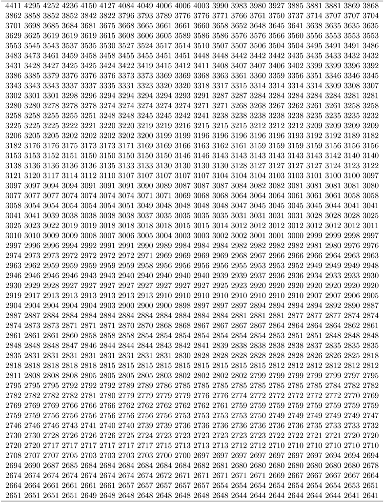
Table 6. Elevations (in feet) of the highest 1000 Simm mountains in the British Isles.

Conflicts of Interest

The author declares no conflicts of interest regarding the publication of this paper.

References

[1]	Pinter, N. and Brandon, M. (1997) How Erosion Builds Mountains. Scientific American, 276, 74-79. https://doi.org/10.1038/scientificamerican0497-74
[2]	Helmholtz (2009) Are the Alps Growing or Shrinking? ScienceDaily, Association of German Research Centres. http://www.sciencedaily.com/releases/2009/11/091105121207.htm
[3]	Champagnac, J., Schlunegger, F., Norton, K., von Blanckenburg, F., Abbühl, L. and Schwab, M. (2009) Erosion-Driven Uplift of the Modern Central Alps. Tectonophysics, 474, 236-249. https://doi.org/10.1016/j.tecto.2009.02.024
[4]	Champagnac, J., Molnar, P., Sue, C. and Herman, F. (2012) Tectonics, Climate, and Mountain Topography. Journal of Geophysical Research, 117, B02403. https://doi.org/10.1029/2011JB008348
[5]	Dielforde, A., Hetzel, R. and Oncken, O. (2020) Megathrust Shear Force Controls Mountain Height at Convergent Plate Margins. Nature, 582, 225-229. https://doi.org/10.1038/s41586-020-2340-7
[6]	Egholm, D., Nielsen, S., Pedersen, V. and Lesemann, J. (2009) Glacial Effects Limiting Mountain Height. Nature, 460, 884-887. https://doi.org/10.1038/nature08263
[7]	Gallen, S., Seymour, N., Glotzbach, C., Stockli, D. and O-Sullivan, P. (2023) Calabrian Forearc Uplift Paced by Slab-Mantle Interactions during Subduction Retreat. Nature Geoscience, 16, 513-520. https://doi.org/10.1038/s41561-023-01185-4
[8]	Wang, K. (2020) Mountain Height Might be Controlled by Tectonic Force, Rather than Erosion. Nature, 582, 189-190. https://doi.org/10.1038/d41586-020-01601-4
[9]	Whipple, K. (2009) The Influence of Climate on the Tectonic Evolution of Mountain Belts. Nature Geoscience, 2, 97-104. https://doi.org/10.1038/ngeo638
[10]	Wolf, S., Huismans, R., Braun, J. and Yuan, X. (2022) Topography of Mountain Belts Controlled by Rheology and Surface Processes. Nature, 606, 516-521. https://doi.org/10.1038/s41586-022-04700-6
[11]	Wikipedia (2022) List of Mountains of the Alps over 4000 Metres. https://en.wikipedia.org/wiki/List_of_mountains_of_the_Alps_over_4000_metres
[12]	Crocker, C. (2022) Database of British and Irish Hills. https://www.hills-database.co.uk/index.html
[13]	Jackson, M. (2009) More Relative Hills of Britain. http://www.rhb.org.uk/humps
[14]	Kendall, S. (2022) Your Basecamp for the World’s Mountains. https://peakery.com
[15]	Maizlish, A. (2003) Prominence and Orometrics. http://www.peaklist.org/theory/theory.html
[16]	Wilson, P. (2001) Listing the Irish hills and Mountains. Irish Geography, 34, 89-95. https://doi.org/10.1080/00750770109555778
[17]	Emberson, R., Hovius, N., Galy, A. and Marc, O. (2016) Chemical Weathering in Active Mountain Belts Controlled by Stochastic Bedrock Landsliding. Nature Geoscience, 9, 42-45. https://doi.org/10.1038/ngeo260
[18]	Hack, J. (1978) Rock Control and Tectonism: Their Importance in Shaping the Appalachian Highlands. U.S.G.S. Report No. 78-403. https://doi.org/10.3133/ofr78403
[19]	He, C., Yang, C., Turowski, J., Rao, G., Roda-Boluda, D. and Yuan, X. (2021) Constraining Tectonic Uplift and Advection from the Main Drainage Divide of a Mountain Belt. Nature Communications, 12, 544-553. https://doi.org/10.1038/s41467-020-20748-2
[20]	Hooke, R. (2003) Time Constant for Equilibration of Erosion with Tectonic Uplift. Geology, 31, 621-624. https://doi.org/10.1130/0091-7613
[21]	Peng, T., Li, Y. and Wu, F. (1977) Tectonic Uplift Rates of the Taiwan Island since the Early Holocene. Memoir of the Geological Society of China, 2, 57-69.
[22]	Simms, A., Rood, D., Rockwell, T. (2020) Correcting MIS5e and 5a Sea-Level Estimates for Tectonic Uplift, an Example from Southern California. Quaternary Science Review, 248, Article ID: 106571. https://doi.org/10.1016/j.quascirev.2020.106571
[23]	White, W. (2009) The Evolution of Appalachian Fluviokarst: Competion between Stream Erosion, Cave Development, Surface Denudation, and Tectonic Uplift, Journal of Cave and Karst Studies, 71, 159-167. https://doi.org/10.4311/jcks2008es0046
[24]	Willenbring, J. and Jerolmack, D. (2016) Steady Rates of Erosion for the Last 10 Ma. Terra Nova, 28, 11-18. https://doi.org/10.1111/ter.12185
[25]	Willett, S., Slingerland, R. and Hovius, N. (2001) Uplift, Shortening, and Steady State Topography in Active Mountain Belts. American Journal of Science, 301, 455-485. https://doi.org/10.2475/ajs.301.4-5.455
[26]	Kloeden, P. and Platen, E. (1992) Numerical Solution of Stochastic Differential Equations, Springer-Verlag, Berlin.
[27]	Allen, E. (2007) Modeling with Itô Stochastic Differential Equations. In: Laubenbacher, R. and Stevens, A., Eds., Mathematical Modelling: Theory and Applications, Springer Dordrecht, Dordrecht. https://doi.org/10.1007/978-1-4020-5953-7
[28]	Allen, E., Allen, L., Arciniega, A. and Greenwood, P. (2008) Construction of Equivalent Stochastic Differential Equation Models. Stochastic Analysis and Applications, 26, 274-297. https://doi.org/10.1080/07362990701857129
[29]	Allen, L. (2010) An Introduction to Stochastic Processes with Applications to Biology. 2nd Edition, CRC Press, Chapman & Hall Publishers, Boca Raton. https://doi.org/10.1201/b12537
[30]	Allen, E. (2016) Environmental Variability and Mean-Reverting Processes. Discrete and Continuous Dynamical Systems, 21, 2073-2089. https://doi.org/10.3934/dcdsb.2016037
[31]	Kladívko, K. (2007) Maximum Likelihood Estimation of the Cox-Ingersoll-Ross process: The MATLAB Implementation. 15th Annual Conference Proceedings of Technical Computing Prague 2007, Praha, 14 November 2007.
[32]	Ortunuga, O. and Ladde, G. (2014) Stochastic Modeling of Energy Commodity Spot Price Processes with Delay in Volatility. American International Journal of Contemporary Research, 4, 1-19.
[33]	Hurn, A., Lindsay, K. and Martin, V. (2003) On the Efficacy of Simulated Maximum Likelihood for Estimating the Parameters of Stochastic Differential Equations. Journal of Time Series Analysis, 24, 45-63. https://doi.org/10.1111/1467-9892.00292
[34]	Misra, D. (2006) Practical Electromagnetics: From Biomedical Sciences to Wireless Communication, John Wiley and Sons, Hoboken. https://doi.org/10.1002/0470054204
[35]	Hogg, R. and Tanis, E. (2001) Probability and Statistical Inference, Prentice Hall, Upper Saddle River. https://doi.org/10.1002/9780470191590
[36]	Blahak, U. (2010) Efficient Approximation of the Incomplete Gamma Function for Use in Cloud Model Applications. Geoscientific Model Development, 3, 329-336. https://doi.org/10.5194/gmd-3-329-2010
[37]	Hoel, P. (1984) Introduction to Mathematical Statistics. 5th Edition, John Wiley and Sons, New York.
[38]	Barakat, H., Nigm, E. and Khaled, O. (2019) Statistical Techniques for Modelling Extreme Value Data and Related Applications, Cambridge Scholars Publisher, Newcastle upon Tyne.
[39]	Schumacher, C., Schwarzenberger, F. and Veselić, I. (2017) A Glivenko-Cantelli Theorem for Almost Additive Functions on Lattices. Stochastic Processes and their Applications, 127, 179-208. https://doi.org/10.1016/j.spa.2016.06.005
[40]	Miškinis, P. (2011) Mathematical Modelling of Mountain Height Distribution on the Earth’s Surface. Geologija, 53, 21-26. https://doi.org/10.6001/geologija.v53i1.1615
[41]	Hsu, C., Chang, C. and Lin, C. (2003) A Practical Guide to Support Vector Classifications. Technical Report, Department of Computer Science and Information Engineering, University of National Taiwan, Taipei, 1-12. https://api.semanticscholar.org/CorpusID:2443126
[42]	Levine, D. (2009) Modeling Tail Behavior with Extreme Value Theory. Risk Management, 17, 14-18.
[43]	Stehlík, M., Aguirre, P., Girard, S., Jordanova, P., Kisel’ák, J., Torres, S., Sadovsky, Z. and Rivera, A. (2017) On Ecosystems Dynamics. Ecological Complexity, 29, 10-29. https://doi.org/10.1016/j.ecocom.2016.11.002
[44]	Zhang, M. and Pan, H. (2021) Application of Generalized Pareto Distribution for Modeling Aleatory Variability of Ground Motion. Natural Hazards, 108, 2971-2989. https://doi.org/10.1007/s11069-021-04809-3
[45]	In Wikipedia (2022) List of Mountains of the British Isles by Height. https://en.wikipedia.org/wiki/List
[46]	Grohmann, C. (2016) Comparative Analysis of Global Digital Elevation Models and Ultra-Prominent Mountain Peaks. ISPRS Annals of the Photogrammetry, Remote Sensing and Spatial Information Sciences, III-4, 12-19. https://doi.org/10.5194/isprs-annals-III-4-17-2016
[47]	Newby, P. (2022) HuMP Bagging List + HuMPs GPS Waypoints. https://www.haroldstreet.org.uk/waypoints
[48]	Scaruffi, P. (2009) Highest Mountains of the World. https://www.scaruffi.com/travel/tallest.html
[49]	In Wikipedia (2022) List of Prominent Mountains of the Alps above 3000 m. https://en.wikipedia.org/wiki/List