Strategies for Advancing Road Construction Slope Stability: Unveiling Innovative Techniques for Managing Unstable Terrain

Guy Oyéniran Adeoti¹, Judicaël Koffi Agbelele^1,2, Crespin Prudence Yabi¹, Rufin Nongnidé Kinhoun¹, Éric Adéchina Alamou¹

¹Laboratory of Testing and Studies in Civil Engineering (L2EGC), National University of Science, Technology, Engineering, and Mathematics (UNSTIM), Department of Zou, Abomey, Republic of Benin.
²National School of Technical Education (ENSET), Lokossa, Republic of Benin.

DOI: 10.4236/ojce.2023.134041                

Abstract

This comprehensive review paper explores various aspects of geotechnical engineering, with a focus on the management of unstable terrains, numerical methods for solving complex soil and consolidation problems, rheological analysis of suspensions and muddy soils, and stability analysis of slopes. It begins by examining the unique physicochemical properties of cohesive sediments, including cohesion and specific surface area. The temporal evolution of deposit concentration and average bed concentration in unstable terrains is discussed, along with settling behavior of isolated particles and hindered settling using empirical equations. Key sedimentation theories, such as Kynch’s theory, and geotechnical consolidation theories, including Terzaghi’s consolidation equation and Gibson’s theory, are presented. The investigation interrelates these theories and principles to offer a holistic view of managing unstable terrains. It also addresses the challenges associated with experimental determination of constitutive relationships and presents alternative simplification methods proposed by researchers. Additionally, it delves into numerical methods for solving nonlinear partial differential equations governing soil behavior, emphasizing the need for numerical frameworks and discussing various techniques and associated challenges. The rheological analysis section covers material flow behavior, rheological behavior models, and the rheological properties of water and cohesive sediment mixtures. Fundamental geotechnical calculations, constitutive laws, and failure criteria are explained, highlighting their relevance in geotechnical engineering applications. This paper provides a multidimensional perspective on geotechnical engineering, offering valuable insights into soil properties, consolidation processes, numerical methods, rheological analysis, and slope stability assessment for professionals in the field.

Keywords

Consolidation Processes, Managing Unstable Terrain, Numerical Methods, Safety Coefficient, Slope Stability Assessment, Soil Cohesion

1. Introduction

In the realm of geotechnical engineering, where the Earth’s intricate structures meet the foundations of human civilization, lies a profound and enduring relationship. The Earth’s materials, ranging from solid bedrock to loose, unstable soils, are the canvas upon which our cities, infrastructure, and societies are built. Understanding and managing these materials is the core mission of geotechnical engineering.

This comprehensive paper embarks on a journey through the multifaceted landscape of geotechnical engineering, with a particular focus on the intricate management of unstable terrains. These terrains, characterized by their variable compositions and behaviors, present both challenges and opportunities for engineers and scientists.

Our exploration commences with an examination of the fundamental properties of cohesive sediments, such as kaolinite, illite, smectite, and chlorite. These microscopic particles, often unseen by the naked eye, hold the key to understanding the macroscopic behaviors of soils. We will delve into their unique physicochemical characteristics, notably cohesion and specific surface area, which have far-reaching implications for geotechnical practice.

The paper’s journey continues by navigating the temporal evolution of deposit concentration and average bed concentration within unstable terrains. These dynamic processes are not mere theoretical abstractions but rather crucial considerations in real-world scenarios. We will also unravel the mysteries of particle settling behavior in quiescent liquids, exploring concepts such as Stokes’ settling velocity and hindered settling described by Richardson and Zaki’s law.

Our path leads us to the heart of sedimentation theories, with a spotlight on the influential Kynch theory. Understanding the relationship between settling velocity and particle concentration is essential for interpreting sedimentation phenomena in geotechnical engineering. This theoretical framework forms the basis for our comprehension of how particles interact and settle in natural and engineered environments.

Consolidation theories, a cornerstone of geotechnical engineering, emerge as a pivotal part of our journey. We will dissect Terzaghi’s consolidation equation and Gibson’s theory, both essential for predicting soil behavior under varying loads and conditions. These theories provide the necessary tools to assess soil settlements and deformation, fundamental aspects of geotechnical design.

However, the strength of this paper lies not only in its ability to dissect individual geotechnical components but also in its capacity to weave them together into a coherent tapestry. The interrelation between sedimentation and consolidation theories will be unveiled, demonstrating how these seemingly distinct concepts merge into a unified framework for managing unstable terrains.

But the challenges in geotechnical engineering are as profound as they are fascinating. We will confront the complexities of experimental determination of constitutive relationships, an endeavor that requires meticulous precision. Furthermore, we will explore innovative simplification methods proposed by visionary researchers, offering practical solutions to these complex challenges.

Our exploration extends to the numerical methods that have revolutionized geotechnical analysis. Finite difference methods and finite element methods are the tools of the trade, enabling engineers to simulate the behavior of soils under various conditions. We will also navigate the intricacies of deformable meshes and discontinuous concentration profiles, underscoring the critical role of numerical frameworks in modern geotechnical practice.

Rheology, the science of material flow behavior, will be our guide through the uncharted waters of suspensions and muddy soils. Stress tensors, strain rates, and rheological laws will come to the forefront as we unravel the mysteries of material flow. Understanding these principles is vital for predicting and managing the complex behavior of soils and sediments in diverse engineering scenarios.

Fundamental geotechnical calculations, constitutive laws, and failure criteria will complete our journey. These concepts are the cornerstone of geotechnical analysis and design, serving as the analytical foundation for engineers seeking to build safe and resilient structures on unstable terrains.

In essence, this paper offers a multidimensional perspective on geotechnical engineering—a discipline where science meets practicality, where the microscopic meets the macroscopic, and where innovation transforms challenges into solutions. As we embark on this expedition through the intricate world beneath our feet, we invite you to join us in unraveling the mysteries of unstable terrains, where knowledge is the compass, and innovation is the guiding star of geotechnical engineering.

2. Innovative Techniques for Managing Unstable Terrain

2.1. Study into Soils and Consolidation of Cohesive Particles in Unstable Terrains

2.1.1. Characterization of Cohesive Particles in Unstable Terrains

A wide variety of soils exists in nature. Sediments can be classified based on their size, origin (marine or fluvial), or physico-chemical properties (especially cohesion). The mineral phase of cohesive sediments is primarily composed of clay minerals, which can be grouped into families: kaolinite, illite, smectite, and chlorite. These minerals possess specific physicochemical properties tied to their structural organization in layers. Generally, finer particles exhibit greater cohesion and higher specific surface area (Table 1).

2.1.2. Experimental Investigation of Soils and Consolidation in Unstable Terrains

Conducting column settlement tests, according to researcher such as Been and Sills (1981), Alexis et al. (1992), Gallois (1995), Masutti (2001) and Alexis et al. (2004) [2] [3] [4] [5] [6] involves introducing a homogenous mixture of solid particles and water into a transparent tube. The initial height and concentration of the mixture are denoted as H₀ and C₀, respectively. Depending on the experimental setup used, the outcomes encompass:

• The evolution of the height (or average concentration) of the sediment deposit,

• Density profiles (which allow deduction of concentration or void ratio profiles),

• Interstitial pressure profiles.

Gamma densimetry and X-ray densimetry (Been and Sills, 1981) are the most commonly employed methods to determine density profiles [2] . They rely on measuring the attenuation of incident rays as they pass through the water/solid particles mixture and require appropriate calibration. They are non-destructive. Note that other methods have been tested or are under development (MRI—Pham Van Bang et al., 2006, ultrasound, electrical properties, for example) [7] .

Using instrumented columns is quite intricate due to numerous experimental challenges that need to be addressed. To acquire density at all levels of the column, a “scanning” from one end to the other is necessary. If measurements aren’t rapid enough, temporal lag can occur, necessitating corrections at times (especially when concentration variations are swift, notably at the beginning of the test). Pressure measurements are also delicate to perform since the pressures at play are low (columns seldom exceed two meters in height). Border effects (at the interface between overlying water and mixture, as well as at the bottom) often skew the density estimation, underscoring the need for constant mass conservation monitoring.

Derived from numerous settlement experiments, Migniot (1968) delineated the subsequent settlement phases (Figure 1) [8] :

Table 1. Geometric characteristics and specific surface areas of key clay families (based on Buffle, 1988) [1] .

Figure 1. Settlement stages of mud (according to Migniot, 1968).

• Flocculation,

• Hindered settling of flocs,

• Initial settlement phase: floc compression,

• Second phase involving the evacuation of interstitial water (accompanied by the formation of preferential drainage pathways),

• A gradual third settlement phase, characterized by the rearrangement of the deposit’s structure and water loss due to compression.

The settlement curves derived from Migniot’s work (Figure 1) illustrate the changes in the average concentration of the sediment. These curves are constructed by plotting the inverse evolution of the interface that demarcates the overlying water and the sediment mixture (Figure 2). The temporal variation of the average sediment concentration, denoted as $C_m\left(t\right)$ , is inversely related to the change in sediment height, $h\left(t\right)$ . This inverse relationship arises from the principle of mass conservation between the initial time and an arbitrary moment, t₁ (Equation (1)):

$H_0\pi r^2{C}_0=h\left(t_1\right)\pi r^2{C}_m\left(t_1\right)$ (1)

where r is the inner radius of the column.

In Figure 2, three settlement phases are discernible:

• During the initial three minutes, the interface remains motionless due to particle flocculation occurring throughout the column.

Figure 2. Settlement curve obtained from Rance sediments; $H_0=50\text{cm}$ and $C_0=50\text{g}/\text{l}$ .

• Between $t=3$ min and $t=30$ min, a clear interface emerges between the mixture and the overlying water. This interface descends at a consistent speed, which is assumed to be the same as that of the flocs located in the upper part of the mixture. As accumulation takes place, a denser deposit forms at the column’s bottom. The concentration at this point is such that flocs experience hindered settling, a result of mutual interference during their descent. Multiple mechanisms contribute to the reduction in floc settling velocity as they amass at the bottom (Winterwerp and Van Kesteren, 2004) [9] . On the suspension scale, the settling flocs induce an upward flow that decelerates the flocs situated above; moreover, the presence of flocs within the fluid alters the suspension’s effective viscosity. At the floc level, interactions (attraction or repulsion) and collisions with other flocs, velocity gradients around the flocs, and wake formation can be observed.

• At $t=30$ min, a distinct transition marks the juncture between the upper part of the developing deposit at the column’s bottom and the interface between overlying water and mixture. Subsequently, the interface’s settling velocity progressively diminishes.

The differentiation among these distinct phases varies based on the material being studied and the initial conditions.

Utilizing X-ray densimetry provides the means to generate concentration profiles akin to those showcased in Figure 3. Within these profiles, distinct zones emerge, each associated with distinct processes. For example, within the profile at $t=1.01$ days, three regions can be discerned:

• In the uppermost segment of the column ( $z>0.43\text{m}$ ), density closely approximates that of water, characterizing the overlying water. This region is demarcated by a pronounced density shift.

• Below the overlying water ( $0.23\text{m}<z<0.43\text{m}$ ), a zone is evident where density remains consistent and closely mirrors the initial density. Here, flocs descend freely with nearly constant velocity, as though they form a single aggregate.

Figure 3. Density profiles; $H_0=0.989\text{m}$ , ${\rho }_0=1068\text{kg}/{\text{m}}^{\text{3}}$ (adapted from Alves, 1992) [10] .

• At the column’s bottom ( $z<0.23\text{m}$ ), a higher-density zone prevails. The thickness of this zone expands as flocs, undergoing constant-rate settling, accumulate at the base. This section of the deposit experiences hindered settling and consolidation.

2.1.3. Theoretical Investigation of Soils and Consolidation in Unstable Terrains

In Migniot’s work (1968) [8] , a proposal is made to describe the temporal evolution of the average deposit concentration, $C_m\left(t\right)$ , through a relationship of the type Equation (2). Upon completion of the settlement process, he presents a concentration distribution along the vertical axis using the formula Equation (3).

$C_m\left(t\right)=A_1\log t+A_2$ (2)

$C\left(t_{fin},z\right)=C\left(h\left(t_{fin}\right)\right)+B_1\log \left(h\left(t_{fin}\right)-z\right)$ (3)

Here, $C\left(h\left(t_{fin}\right)\right)$ denotes the concentration at the interface, while A₁, A₂, and B₁ stand for empirical coefficients.

In the approach put forth by Hayter (1986) [11] , the ultimate deposit concentration as well as the final consolidation time, $t_{fin}$ , are assumed to vary linearly with C₀ (Equation (4)). Additionally, the average bed concentration is characterized by the empirical relationship Equation (5). The distribution within the bed is provided by the empirical formula Equation (6).

$\{\begin{array}{l}{C}_m\left(t_{fin}\right)=A_1+A_2{C}_0\\ t_{fin}=B_1+B_2{C}_0\end{array}$ (4)

$\frac{C_m\left(t\right)}{C_m\left(t_{fin}\right)}=1-D_1\exp \left(-\frac{D_2\cdot t}{t_{fin}}\right)$ (5)

$\frac{C\left(z,t\right)}{C_m\left(t\right)}=E_1{\left(\frac{h\left(t\right)-z}{h\left(t\right)}\right)}^{E_2}$ (6)

In this context, $A_i$ , $B_i$ , $D_i$ , and $E_i$ denote empirical constants, while $C_m\left(t_{fin}\right)$ stands for the average deposit concentration upon completion of the consolidation process.

Stokes’ law

When an isolated particle falls in a quiescent liquid, its settling velocity $W_s$ can be determined by considering the balance of forces acting upon it: gravity, buoyancy, and drag. This leads to the Stokes settling velocity for isolated particles, denoted as $W_{Stokes}$ (Equation (7)) [12] :

$W_{Stokes}=\frac{g{D}^2}{18\nu }\frac{{\rho }_s-{\rho }_w}{{\rho }_w}$ (7)

where D stands for the particle diameter in micrometers, $\nu$ denotes the kinematic viscosity of the fluid, ${\rho }_s$ and ${\rho }_w$ respectively represent the mass densities of the solid particles and the fluid, and g signifies gravity.

For particle diameters exceeding 50 μm, the Oseen’s law [13] proves more applicable than the Stokes’ law. The Oseen settling velocity is formulated as (Equation (8)):

$W_{Stokes}=\frac{4\nu }{3D}\left(-1+\sqrt{1+\frac{{\rho }_s-{\rho }_w}{{\rho }_w}\frac{g{D}^3}{12{\nu }^2}}\right)$ (8)

Zaki’s law

An equation of the type Equation (9) is commonly utilized to characterize the decrease in particle settling velocity as the concentration rises under the influence of hindered settling. This extends the empirical Richardson and Zaki’s law (1954) [14] , with $A_1=1$ .

$W_S=W_{Stokes}{\left(1-A_1{\varphi }_S\right)}^{A_2}$ (9)

Here, ${\varphi }_S$ signifies the solid volume fraction, and A₁ and A₂ are constants fine-tuned through experimentation.

Kynch theory

The Kynch theory (1952) [15] holds a prominent position among sedimentation theories. Its primary assumption is that the settling velocity of particles (assumed to be identical), V_S, is solely dependent on the particle concentration, C. The mixture is considered to be horizontally uniform. The equation for mass conservation is expressed as (Equation (10)):

$\frac{\partial C}{\partial t}+\frac{\partial C{V}_S\left(C\right)}{\partial z}=0$ (10)

where t represents time and z is the vertically oriented axis directed upwards. Upon incorporating the solid flux S, Equation (10) is modified to Equation (11):

$\frac{\partial C}{\partial t}+\frac{\partial S}{\partial z}=0$ (11)

Equation (11) can be rewritten as Equation (12) or Equation (13) by substituting Equation (14).

$\frac{\partial C}{\partial t}+\frac{\partial S}{\partial C}\frac{\partial C}{\partial z}=0$ (12)

$\frac{\partial C}{\partial t}+V\left(C\right)\frac{\partial C}{\partial z}=0$ (13)

$V\left(C\right)=\frac{\partial S}{\partial C}$ (14)

Equation (10) constitutes a hyperbolic equation. It represents a first-order wave equation that can be comprehended by postulating that C propagates at a velocity $V\left(C\right)$ . To put it differently, a concentration layer C situated at time t and at a level z will relocate to a level $z+V\left(C\right)\Delta t$ at time $t+\Delta t$ .

Kynch presents a visual interpretation (Figure 4) of this equation through the lens of a graph $\left(x\mathrm{<mo>\; ;\; </mo>}t\right)$ . He discerns three domains:

• Within the OAB zone, concentrations remain constant, and isoconcentration lines run parallel. In this sector of the graph, particle settling velocity remains steady.

• In the OBC zone, the gradient of isoconcentration lines fluctuates. This segment of the graph corresponds to hindered settling, wherein the pace of concentration variation is determined by the slope of the isoconcentration line.

• Beneath the OCD zone, the maximum compaction concentration is achieved, signifying the cessation of particle evolution.

2.1.4. Geotechnical Approach of Consolidation in Unstable Terrains

The concept of gel concentration, also known as structural concentration, defines the threshold at which a transition occurs between a suspension (where flocs are supported by the fluid) and a deposit that exhibits a structured phase. In simpler terms, it signifies the concentration at which the flocs become so closely packed that they form a continuous three-dimensional network.

When this loosely organized network experiences the tendency to collapse due to its own weight, a rearrangement of its structure takes place. This rearrangement enables the structure to promptly bear partial weight from the grains of the upper layers. Consequently, the total vertical stress becomes lower than the interstitial pressure, indicating the emergence of effective stresses, denoted as ${\sigma }^{\prime }$ . Terzaghi introduced the concept of effective stresses as the portion of total stress that is transmitted through the grains.

Figure 4. Isoconcentration lines (adapted from Kynch, 1952).

The appearance of effective stresses signifies the pivotal transition from sedimentation to consolidation.

Theory of Terzaghi The equation of Terzaghi (1943) (Equation (15)) [16] , cherished by soil mechanics experts, is founded on the assumption of small deformations and the following hypotheses:

• The soil is uniform and fully saturated,

• Both water and grains are incompressible,

• Consolidation occurs in one dimension,

• Darcy’s law is valid,

• The mechanical properties of the soil remain constant, and the relationship ${\sigma }^{\prime }\left(e\right)$ is linear.

Terzaghi’s consolidation equation is well-suited to describe the latter phases of the consolidation process, namely when deformations become minor.

$\frac{\partial {\sigma }^{\prime }}{\partial t}-C_V\frac{{\partial }^2{\sigma }^{\prime }}{{\partial }^{2}z}=0$ (15)

where C_V is the coefficient of consolidation, which can be determined through an oedometer test.

Gibson’s theory Gibson’s theory (1967) [17] stands as a fundamental reference in the realm of consolidation by researchers such as Toorman (1999); Winterwerp (1999); Merckelbach (2000); Bartholomeeusen (2003); and others [18] [19] [20] [21] . The Gibson equation is expressed as (Equation (16)):

$\frac{\partial e}{\partial t}+{\left(1+e\right)}^2\frac{{\rho }_s-{\rho }_w}{{\rho }_w}\frac{\partial }{\partial z}\left(\frac{k}{{\left(1+e\right)}^2}\right)+\frac{{\left(1+e\right)}^2}{g\cdot {\rho }_w}\frac{\partial }{\partial z}\left(\frac{k}{1+e}\frac{\partial {\sigma }^{\prime }}{\partial z}\right)=0$ (16)

where e represents void ratio and k is the soil permeability.

Since the sediment is fully saturated with water, the intermediary equations that lead to the Gibson equation can be formulated using sediment concentrations instead of void ratios (Equation (17)). These equations amount to four: Terzaghi’s postulate, Darcy’s law, the continuity equation, and the mass conservation equation.

As per Terzaghi’s postulate (Equation (18)), the total stress generated by the weight of the water and grains is borne by the interactions among the grains (the solid framework of the sediment) and by the interstitial water pressures u.

Interstitial pressures can be broken down into a hydrostatic component denoted as $u_h$ and a component known as interstitial excess pressure denoted as $p_e$ (Equation (19)).

$C=\frac{{\rho }_s}{1+e}$ (17)

$\sigma ={\sigma }^{\prime }+u$ (18)

$u=u_h+p_e$ (19)

The Darcy’s law (1856) [22] , as expressed by Equation (20), serves to describe the dissipation of interstitial excess pressures. Consolidation is considered complete when these excess pressures are entirely dissipated, meaning that the interstitial pressure becomes hydrostatic.

$\frac{{\rho }_s-C}{{\rho }_s}\left(V_f-V_s\right)=-k\left(C\right)\frac{1}{g\cdot {\rho }_w}\frac{\partial p_e}{\partial z}$ (20)

where $V_s$ and $V_f$ are the respective vertical velocities of solid particles and the fluid relative to a reference plane (see Figure 5). The continuity equation is formulated as (Equation (21)):

$\left({\rho }_s-C\right)V_f+C{V}_s=0$ (21)

The conservation of mass is formulated as (Equation (22)):

$\frac{\partial C}{\partial t}+\frac{\partial V_{s}C}{\partial z}=0$ (22)

By integrating the equations of continuity, Darcy’s law, and Terzaghi’s postulate, we arrive at an expression for the velocity of solid particles, denoted by Equation (23).

$V_s=k+\frac{k}{g\cdot {\rho }_w}\left(\frac{\partial \sigma }{\partial z}+\frac{\partial {\sigma }^{\prime }}{\partial z}\right)$ (23)

The assumptions underlying Gibson’s theory are as follows:

• Permeability and effective stresses depend solely on concentration,

• The medium is fully saturated,

• Darcy’s law is applicable,

• Consolidation is a one-dimensional process,

• The deposit is uniform on a horizontal plane.

2.1.5. Effective Stress

The relationships describing the changes in effective stresses and permeability concerning void ratios (or concentration) can be experimentally ascertained using the approach outlined by Been and Sills (1981) [2] . This method involves deducing $k\left(e\right)$ through Equation (24), derived from Darcy’s law and the continuity equation. $V_s$ is estimated by measuring the displacement of a specific point within the deposit over a time interval between two concentration profiles,

Figure 5. Conventions.

and i is determined from pressure profiles. For the determination of ${\sigma }^{\prime }\left(e\right)$ ( ${\sigma }^{\prime }\left(C\right)$ ), Terzaghi’s postulate is applied. u is directly obtained from interstitial pressure measurements, and $\sigma$ is determined from concentration profiles using Equation (25).

$k=-V_{s}i$ (24)

where i denotes the hydraulic gradient.

$\sigma \left(z\right)=g\left(\frac{\rho s-C}{{\rho }_s}{\rho }_w+C\right)\left(h-z\right)$ (25)

where h denotes the water/sediment interface level.

By proceeding in this manner, one obtains clouds of points ( $k\left(e\right)$ and ${\sigma }^{\prime }\left(e\right)$ ) that are more or less compact (Figure 6 and Figure 7). Using these data points, a least squares regression is conducted to determine the empirical coefficients $A_i$ and $B_i$ , which are then incorporated into a priori functions as presented below (Bartholomeeusen et al., 2002) (Equation (26) & Equation (27)) [23] :

$\{\begin{array}{ll}e=A_1\ln \left(k\right)+A_2\hfill & \mathrm{<mtext>\; \hspace{0.17em}\; </mtext>\; <mtext>\; \hspace{0.17em}\; </mtext>\; <mtext>\; \hspace{0.17em}\; </mtext>}(\text{a})\hfill \\ k=A_1{\text{e}}^{A_2}\hfill & \mathrm{<mtext>\; \hspace{0.17em}\; </mtext>\; <mtext>\; \hspace{0.17em}\; </mtext>\; <mtext>\; \hspace{0.17em}\; </mtext>}(\text{b})\hfill \\ k=A_1{\varphi }_s^{A_2}\hfill & \mathrm{<mtext>\; \hspace{0.17em}\; </mtext>\; <mtext>\; \hspace{0.17em}\; </mtext>\; <mtext>\; \hspace{0.17em}\; </mtext>}(\text{c})\hfill \\ k=\exp \left(-A_1+A_{2}e\right)\hfill & \mathrm{<mtext>\; \hspace{0.17em}\; </mtext>\; <mtext>\; \hspace{0.17em}\; </mtext>\; <mtext>\; \hspace{0.17em}\; </mtext>}(\text{d})\hfill \end{array}$ (26)

$\{\begin{array}{ll}e=-B_1{{\sigma }^{\prime }}^{B_2}+B_3\hfill & \mathrm{<mtext>\; \hspace{0.17em}\; </mtext>\; <mtext>\; \hspace{0.17em}\; </mtext>\; <mtext>\; \hspace{0.17em}\; </mtext>\; <mtext>\; \hspace{0.17em}\; </mtext>}(\text{a})\hfill \\ {\sigma }^{\prime }=B_1{\varphi }_s^{B_2}\hfill & \mathrm{<mtext>\; \hspace{0.17em}\; </mtext>\; <mtext>\; \hspace{0.17em}\; </mtext>\; <mtext>\; \hspace{0.17em}\; </mtext>\; <mtext>\; \hspace{0.17em}\; </mtext>}(\text{b})\hfill \\ e=B_1{\left({\sigma }^{\prime }+B_2\right)}^{B_3}\hfill & \mathrm{<mtext>\; \hspace{0.17em}\; </mtext>\; <mtext>\; \hspace{0.17em}\; </mtext>\; <mtext>\; \hspace{0.17em}\; </mtext>\; <mtext>\; \hspace{0.17em}\; </mtext>}(\text{c})\hfill \end{array}$ (27)

Figure 6. $e\left(k\right)$ relationships for various sediments (adapted from Bartholomeeusen, 2003).

Figure 7. $e\left({\sigma }^{\prime }\right)$ relationships for different sediments (adapted from Bartholomeeusen, 2003).

Various challenges can arise when attempting to establish constitutive relationships using the method proposed by Been and Sills (1981):

• The ${\sigma }^{\prime }\left(C\right)$ relationship is influenced by initial conditions. This is due to the thixotropic nature of sediments, where the structural arrangement of a deposit depends on its formation history (i.e., the assumption that effective stresses depend solely on C is sometimes difficult to apply);

• Equipped columns might not be accessible in all research facilities;

• Achieving satisfactory precision in density and pressure profiles can be difficult due to experimental constraints related to such measurements: limited accuracy of pressure sensors, edge effects, signal noise, etc.;

• Estimating V_s is also complex. For low concentrations, a minor variation in C results in a significant change in V_s (and consequently k). Furthermore, variability in V_s (and thus k) is often substantial as a limited number of sediment treatments can hinder the achievement of reliable low-concentration tests.

To address the variability in experimentally determined $k\left(C\right)$ and ${\sigma }^{\prime }\left(C\right)$ relationships, a substantial number of measurements are usually carried out.

Given this situation, Merckelbach and Kranenburg (2004) [24] introduced a technique to determine constitutive relationships based on straightforward settlement curves. This type of experimental data is much simpler to obtain since it requires minimal resources (no pressure or density measurements are necessary). Their approach involves determining the parameters introduced into the constitutive relationships (the $A_i$ and $B_i$ in Equation (26) and Equation (27)) in a manner that aligns the calculated settlement curve using Gibson’s theory, $h_{cal}\left(A_i\mathrm{,}{B}_i\mathrm{,}t\right)$ , with the experimental settlement curve, $h_{exp}\left(t\right)$ . In essence, they solve Equation (28).

$\left(A_i\mathrm{,}{B}_i\right)=\underset{A_i\mathrm{,}{B}_i}{\min }\left(h_{cal}\left(A_i\mathrm{,}{B}_i\mathrm{,}t\right)-h_{exp}\left(t\right)\right)$ (28)

In order to derive an analytical expression for $h_{cal}\left(A_i\mathrm{,}{B}_i\mathrm{,}t\right)$ , Merckelbach and Kranenburg (2004) adopt a two-phase approach where simplifying assumptions can be applied.

Initially, the $A_i$ coefficients are determined by focusing solely on the first phase of a sedimentation/consolidation test, as during this part of the test:

• Interstitial water expulsion is the dominant phenomenon (implying the significant role of permeability),

• The impact of effective stresses can be disregarded.

By neglecting effective stresses, the Gibson equation simplifies and transforms into a wave equation that has an analytical solution. Through integration, an expression for the deposit height $h_{cal}\left(A_i\mathrm{,}t\right)$ can be obtained, enabling the solution of Equation (29). In this step, Merckelbach and Kranenburg assume a permeability law in the form of Equation (26)(c).

$A_i=\underset{A_i}{\min }\left(h_{cal}\left(A_i,t\right)-h_{exp}\left(t\right)\right)\forall ttq{\sigma }^{\prime }\approx 0$ (29)

To determine the $B_i$ coefficients, Merckelbach and Kranenburg make the assumption that the effective stress law takes the form of Equation (26)(b) with $B_i=A_2$ . Consequently, there remains only one coefficient to be determined: $B_1$ . When considering equilibrium ( $\partial C/\partial t=0$ ), the Gibson equation simplifies to (Equation (30)):

$\frac{{\rho }_s-{\rho }_w}{{\rho }_w}C=-\frac{{\rho }_s}{g\cdot {\rho }_w}\frac{\partial {\sigma }^{\prime }}{\partial z}$ (30)

By integrating Equation (30), an analytical expression for $h_{cal}\left(B_1\mathrm{,}{t}_{fin}\right)$ at equilibrium ( $t_{fin}$ being the time needed to reach equilibrium) can be obtained. This enables the determination of $B_1$ in such a way that the equality $h_{cal}\left(B_1\mathrm{,}{t}_{fin}\right)=h_{exp}\left(t_{fin}\right)$ is satisfied.

However, it’s important to note that the method proposed by Merckelbach and Kranenburg may not always be applicable due to certain limitations. The choice of constitutive relationships is constrained by the need for easily integrable laws to derive simple analytical expressions. Moreover, the number of coefficients that can be calculated is limited to three, which enforces the assumption $B_2=A_2$ that may not hold in all cases.

2.1.6. Interrelation of Soils and Consolidation Theories in Unstable Terrains

Gibson’s theory represents a broader perspective stemming from the works of Kynch and Terzaghi (1943) as discussed by Winterwerp and Van Kesteren (2004) [9] .

In fact, by neglecting effective stresses, the velocity of solid particles conforms to Equation (31), resulting in Equation (33) as derived from Equation (32)

$V_s=k\left(C\right)+\frac{k\left(C\right)}{g\cdot {\rho }_w}\left(\frac{\partial \sigma }{\partial z}\right)$ (31)

$\frac{\partial \sigma }{\partial z}=g\left(\left(\frac{C}{{\rho }_s}-1\right){\rho }_w-C\right)$ (32)

$V_s=V_s\left(C\right)=k\left(C\right)C\left(\frac{1}{{\rho }_s}-\frac{1}{{\rho }_w}\right)$ (33)

Upon incorporating Equation (33) into Equation (22), the resulting Equation (34) represents an equivalent formulation to that of Kynch (1952). Expanding on this principle, Pane and Schiffman (1985) [25] introduce a generalization of the Terzaghi principle with the relationship Equation (35), allowing them to characterize sedimentation and consolidation using a unified approach.

$\frac{\partial C}{\partial t}+\frac{\text{d}{V}_s\left(C\right)C}{\text{d}C}\frac{\partial C}{\partial z}=0$ (34)

$\sigma =\beta \left(C\right){\sigma }^{\prime }+u$ (35)

Here, $\beta \left(C\right)$ takes the value of 1 when $C>C_t$ and 0 otherwise, where $C_t$ signifies the concentration denoting the sedimentation-consolidation transition.

The assumptions employed within Terzaghi’s theory (1943) allow for the omission of the advection term from Equation (16), resulting in its reduction to either Equation (36) or Equation (37). In this context, we indeed observe an equation akin to Equation (15), achievable by adopting a consolidation coefficient like that described in Equation (39).

$\frac{\partial e}{\partial t}+\frac{{\left(1+e\right)}^2}{g\cdot {\rho }_w}\frac{\partial }{\partial z}\left(\frac{k}{1+e}\frac{\partial {\sigma }^{\prime }}{\partial z}\right)=0$ (36)

$\frac{\partial e}{\partial t}+\frac{\left(1+e\right)k}{g\cdot {\rho }_w}\frac{{\partial }^2{\sigma }^{\prime }}{{\partial }^{2}z}=0$ (37)

$\frac{\partial {\sigma }^{\prime }}{\partial t}-C_v\frac{{\partial }^2{\sigma }^{\prime }}{{\partial }^{2}z}=0$ (38)

$C_V=-\frac{k\left(1+e\right)}{g\cdot {\rho }_w}\frac{\partial {\sigma }^{\prime }}{\partial e}$ (39)

2.1.7. Numerical Methods

Realistic theories of soils and consolidation rely on nonlinear partial differential equations that lack analytical solutions. Therefore, a numerical framework must be established to obtain approximate solutions to the problem at hand. Sedimentation equations (hyperbolic equations) are typically addressed through finite difference methods by Bürger and Hvistendahl (2001) [26] or finite volume methods (such as the first-order upstream scheme or the second-order Lax-Wendroff scheme). Consolidation equations, which take the form of convection/diffusion equations, are commonly tackled using finite element methods (for instance, Rouas (1996) [27] or finite differences (including Le Normant (2000) [28] ).

In the realm of numerical solutions, two challenges arise when dealing with equations like Gibson’s. Firstly, the mesh used to compute the variable describing the deposit’s evolution ( $e\left(z\mathrm{,}t\right)$ , $C\left(z\mathrm{,}t\right)$ , or ${\varphi }_s\left(z\mathrm{,}t\right)$ ) must be “deformable,” as it spans from the fixed bed ( $z=0$ ) to the mobile water-deposit interface. The Lagrangian approach is often employed in this context. Consequently, the Gibson equation can be expressed in the following form (Equation (40)):

$\frac{\partial e}{\partial t}+\frac{{\rho }_s-{\rho }_w}{{\rho }_w}\frac{\text{d}}{\text{d}e}\left(\frac{k}{1+e}\right)\frac{\partial e}{\partial \Omega }+\frac{\partial }{\partial \Omega }\left(\frac{k}{\left(1+e\right){\rho }_w\cdot g}\frac{\text{d}{\sigma }^{\prime }}{\text{d}e}\frac{\partial e}{\partial \Omega }\right)=0$ (40)

With

$\Omega \left(z\mathrm{,}t\right)={\displaystyle {\int }_0^z}\frac{\text{d}{z}^{\prime }}{1+e\left(z^{\prime }\mathrm{,}t\right)}$ (41)

Another complexity arises due to the presence of discontinuous concentration profiles, which can lead to numerical oscillations.

A distinct approach to the issue involves treating the water/sediment mixture as a medium comprised of two interacting phases. Through this method, conservation equations for mass and momentum are established for each of the phases by researchers like Toorman (1996); Lee et al. (2000); Bürger (2000); … [29] [30] [31] .

2.1.8. Rheological Analysis of Suspensions and Muddy Soils

Rheology is the science that deals with the flow behavior of materials, encompassing the characterization of substances ranging from fluids to deformable solids. Comprehensive resources on the topic include Midoux’s work (1985) [32] and the contributions of Coussot and Grossiord (2002) [33] , as well as the thorough thesis by Besq (2000) [34] .

In rheology, the stress state at a point within the material is expressed using a two-dimensional symmetric tensor known as the Cauchy stress tensor. It is commonly denoted as $\overline{\stackrel{¯}{\sigma }}$ or ${\sigma }_{ij}$ (Equation (42)). This tensor can be split into an isotropic term $p\overline{\stackrel{¯}{I}}$ and a component referred to as the stress deviator, indicated by $\overline{\stackrel{¯}{\tau }}$ .

$\overline{\stackrel{¯}{\sigma }}=p\overline{\stackrel{¯}{I}}+\overline{\stackrel{¯}{\tau }}$ (42)

Here, p denotes the average isotropic pressure, and $\overline{\stackrel{¯}{I}}$ represents the unit diagonal tensor.

When flow takes place, the constituents of the fluid move relative to each other, resulting in the emergence of velocity gradients. From the velocity gradient tensor $\nabla \stackrel{\to }{u}$ , the tensor of strain rates, indicated as $\overline{\stackrel{¯}{D}}$ , can be derived using Equation (43):

$\overline{\stackrel{¯}{D}}=\frac{1}{2}\left(\nabla \stackrel{\to }{u}+{\left(\nabla \stackrel{\to }{u}\right)}^{\text{T}}\right)$ (43)

where $\stackrel{\to }{u}$ denotes the flow velocity.

Commonly, rheological laws are expressed by relating the stress deviator $\overline{\stackrel{¯}{\tau }}$ to the tensor of strain rates $\overline{\stackrel{¯}{D}}$ . As an illustration, the most straightforward constitutive law is derived for a Newtonian fluid (Equation (44)).

$\overline{\stackrel{¯}{\tau }}=2\mu \overline{\stackrel{¯}{D}}$ (44)

Here, $\mu$ denotes the fluid’s viscosity.

Characterizing a law such as Equation (44) experimentally can be challenging. To determine the rheological properties of a fluid, one often starts with simple cases where the relationships between $\overline{\stackrel{¯}{\tau }}$ and $\overline{\stackrel{¯}{D}}$ can be simplified. For instance, in simple shear, $\overline{\stackrel{¯}{\tau }}$ and $\overline{\stackrel{¯}{D}}$ are expressed as follows (Equation (45) and Equation (46)):

$\overline{\stackrel{¯}{\tau }}=\left[\begin{array}{ccc}{\sigma }_{xx}& {\tau }_{xy}& 0\\ {\tau }_{xy}& {\sigma }_{yy}& 0\\ 0& 0& {\sigma }_{zz}\end{array}\right]$ (45)

$\overline{\stackrel{¯}{D}}=\frac{\stackrel{\dot{}}{\gamma }}{2}\left[\begin{array}{ccc}0& 1& 0\\ 1& 0& 0\\ 0& 0& 0\end{array}\right]$ (46)

where $\stackrel{\dot{}}{\gamma }$ denotes the shear rate or velocity gradient, and ${\tau }_{xy}$ is the shear stress, which will be denoted as $\tau$ throughout the manuscript.

The apparent viscosity is defined as: $\eta =\tau /\stackrel{\dot{}}{\gamma }$

Rheometric tests aim to establish the relationship between the scalar quantities $\tau$ and $\stackrel{\dot{}}{\gamma }$ , which is referred to as a rheogram. Several mathematical models have been proposed to describe the most commonly encountered rheological behaviors. However, these models are generally only valid under specific flow conditions. Here are a few examples:

• For a Newtonian fluid in simple shear, we have: $\tau =\mu \stackrel{\dot{}}{\gamma }$ .

• For a shear-thinning (Rheofluidification which results from material destabilization caused by fluid shear) fluid, a power-law model is often used: $\tau =k{\stackrel{\dot{}}{\gamma }}^n$ with $n<1$ . In this case, the apparent viscosity $\eta =k{\stackrel{\dot{}}{\gamma }}^{n-1}$ decreases as $\stackrel{\dot{}}{\gamma }$ increases.

• For a yield-stress fluid, which means a fluid that only flows when the applied stress surpasses a critical value ${\tau }_y$ , the flow curve is expressed as (Equation (47)):

$\{\begin{array}{ll}\tau ={\tau }_y+f\left(\stackrel{\dot{}}{\gamma }\right)\hfill & \text{if}\tau >{\tau }_y\hfill \\ \stackrel{\dot{}}{\gamma }=0\hfill & \mathrm{<mtext>\; \hspace{0.17em}\; </mtext>}\text{if}\tau \le {\tau }_y\hfill \end{array}$ (47)

For Bingham fluids, the relationship is given by $f\left(\stackrel{\dot{}}{\gamma }\right)={\eta }_{pl}\stackrel{\dot{}}{\gamma }$ , where ${\eta }_{pl}$ represents the plastic viscosity. In the case of Herschel-Bulkley fluids, the relation becomes $f\left(\stackrel{\dot{}}{\gamma }\right)=k{\stackrel{\dot{}}{\gamma }}^n$ .

All these aforementioned laws are illustrated in Figure 8.

Figure 8. Foundational rheological behavior laws.

Mixtures consisting of water and cohesive sediments exhibit intricate rheological properties. Notable rheological investigations pertaining to sediments encompass studies conducted by Toorman (1992), Babatope et al. (2006), and Besq and Makhloufi (2007) [35] [36] [37] .

A suspension can be treated as Newtonian as long as its sediment concentration remains low (

Muddy deposits also manifest rheofluidification and thixotropy. Thixotropy denotes that, at a given stress level, the rheological demeanor of a deposit may evolve over time. This quality stems from the disruption of inter-floc or inter-particle bonds due to shear and the material’s capacity to restructure while at rest.

2.2. Fundamentals of Geotechnical Calculations

Much like in rheology, the cornerstone of geotechnical calculations is the mechanics of continuous mediums. However, the behavioral laws of soils are unique to the geotechnical realm. The publication by Nova (2005) [38] thoroughly outlines the fundamentals of geotechnical computations.

The mathematical characterization of soils employs the notion of stress tensor (Equation (42)). The geotechnicians’ concept of effective stresses entails considering the relationship presented by Equation (48), where the term for effective pressures, $p^{\prime }$ , equals $p-u$ , where u represents interstitial water pressures. The strain tensors are formulated as delineated in Equation (49).

${{\sigma }^{\prime }}_{ij}=p^{\prime }{\delta }_{ij}+{{\tau }^{\prime }}_{ij}$ (48)

where ${\delta }_{ij}$ denotes the Kronecker symbol.

$\overline{\stackrel{¯}{\epsilon }}=\left[\begin{array}{ccc}{\epsilon }_{xx}& \frac{1}{2}{\gamma }_{xy}& \frac{1}{2}{\gamma }_{xz}\\ \frac{1}{2}{\gamma }_{yx}& {\epsilon }_{yy}& \frac{1}{2}{\gamma }_{yz}\\ \frac{1}{2}{\gamma }_{zx}& \frac{1}{2}{\gamma }_{zy}& {\epsilon }_{zz}\end{array}\right]$ (49)

Given that the stress tensor is symmetric, there exists an orthonormal frame in which the matrix becomes diagonal. The three corresponding directions are the principal stress directions, and the eigenvalues are referred to as principal stresses, denoted as ${\sigma }_1$ , ${\sigma }_2$ , and ${\sigma }_3$ .

Each soil element Ω must maintain equilibrium under the influence of its individual weight and the forces transmitted by neighboring soil elements. This necessitates the fulfillment of equilibrium equations, as indicated by Equation (50):

$\{\begin{array}{l}\frac{\partial {\sigma }_{xx}}{\partial x}+\frac{\partial {\tau }_{yx}}{\partial y}+\frac{\partial {\tau }_{zx}}{\partial z}=0\\ \frac{\partial {\tau }_{xy}}{\partial x}+\frac{\partial {\sigma }_{yy}}{\partial y}+\frac{\partial {\tau }_{zy}}{\partial z}=0\\ \frac{\partial {\tau }_{xz}}{\partial x}+\frac{\partial {\tau }_{yz}}{\partial y}+\frac{\partial {\tau }_{zz}}{\partial z}+{\gamma }_{soil}=0\end{array}$ (50)

where ${\gamma }_{soil}$ denotes the weight of a soil element.

The kinematic conditions encompass geometric relationships linking deformations to displacements $U_i\left(i=x,y,z\right)$ . These relations can be formulated as (Equation (51) and Equation (52)):

$\{\begin{array}{l}{\epsilon }_{xx}=\frac{\partial U_x}{\partial x}\\ {\epsilon }_{yy}=\frac{\partial U_y}{\partial y}\\ {\epsilon }_{zz}=\frac{\partial U_z}{\partial z}\end{array}$ (51)

$\{\begin{array}{l}{\epsilon }_{xy}=\frac{1}{2}{\gamma }_{xy}=\frac{1}{2}\left(\frac{\partial U_x}{\partial y}+\frac{\partial U_y}{\partial x}\right)\\ {\epsilon }_{xz}=\frac{1}{2}{\gamma }_{xz}=\frac{1}{2}\left(\frac{\partial U_x}{\partial z}+\frac{\partial U_z}{\partial x}\right)\\ {\epsilon }_{yz}=\frac{1}{2}{\gamma }_{yz}=\frac{1}{2}\left(\frac{\partial U_y}{\partial z}+\frac{\partial U_z}{\partial y}\right)\end{array}$ (52)

2.2.1. Behavioral Law

A constitutive law establishes a connection between the stresses and deformations experienced by the soil, as described in Equation (53). Soil behavior is highly intricate since it depends on factors such as the loading history, saturation level, and loading rate. Furthermore, it is generally irreversible and nonlinear. No mathematical model can fully encompass all the characteristics of a soil.

To determine the deformations experienced by soil when subjected to stress, it is necessary to integrate Equation (53), which requires specifying an initial stress state. This state is typically determined by considering the weight of the soil as homogeneous, isotropic, and saturated. Vertical pressures are assumed to be hydrostatic. Regarding horizontal pressures, two scenarios can arise. In the case of undisturbed soil (that has not undergone significant decompression due to erosion, excavation, etc.), the ratio between horizontal and vertical pressures is assumed constant and denoted as K₀, which represents the coefficient of at-rest pressure. For soil that is not undisturbed (having experienced considerable erosion over its history, for example), the ratio is no longer constant, and the concept of overconsolidation comes into play (denoted by OCR, the overconsolidation ratio).

$\frac{\partial }{\partial t}\overline{\stackrel{¯}{\epsilon }}=\overline{\stackrel{¯}{S}}\frac{\partial }{\partial t}\overline{\stackrel{¯}{{\sigma }^{\prime }}}$ (53)

where $\overline{\stackrel{¯}{S}}$ is a tensor known as the compliance tensor.

2.2.2. Elasticity

For a linear elastic isotropic material, the connection between stresses and strains can be characterized using the generalized Hooke’s law, represented as Equation (54) in vector form. It’s worth noting that $\nu =0.5$ corresponds to a scenario where the material is incompressible. While this law is linear and doesn’t consider irreversibility or stress path dependency, it may not be directly applicable to geotechnical applications. Nevertheless, it can yield valuable insights during the preliminary stages of a project according to Mestat (1998) [39] [40] .

$\left[\begin{array}{c}{\epsilon }_{xx}\\ {\epsilon }_{yy}\\ {\epsilon }_{zz}\\ {\gamma }_{xy}\\ {\gamma }_{xz}\\ {\gamma }_{yz}\end{array}\right]=\frac{1}{E}\cdot \left[\begin{array}{cccccc}1& -\nu & -\nu & 0& 0& 0\\ -\nu & 1& -\nu & 0& 0& 0\\ -\nu & -\nu & 1& 0& 0& 0\\ 0& 0& 0& 2\left(1+\nu \right)& 0& 0\\ 0& 0& 0& 0& 2\left(1+\nu \right)& 0\\ 0& 0& 0& 0& 0& 2\left(1+\nu \right)\end{array}\right]\cdot \left[\begin{array}{c}{\sigma }_{xx}\\ {\sigma }_{yy}\\ {\sigma }_{zz}\\ {\tau }_{xy}\\ {\tau }_{xz}\\ {\tau }_{yz}\end{array}\right]$ (54)

where E represents the Young’s modulus and $\nu$ denotes the Poisson’s ratio.

2.2.3. Elasto-Plasticity

Upon reaching a specific stress threshold, soil experiences both reversible elastic deformations and irreversible plastic deformations, which signify a disruption in the soil structure.

The plasticity function f is a scalar function that, depending on the stress state and material history, determines whether a specific load variation induces plastic or elastic deformations. It can be formulated as (Equation (55)):

$f=f\left(\overline{\stackrel{¯}{{\sigma }^{\prime }}}\mathrm{,}{\psi }_1\right)\le 0$ (55)

where ${\psi }_1$ is a vector that depends on the history of plastic deformations (allowing for considerations such as strain hardening, for example).

In cases of low mechanical loads, f is strictly negative. In this scenario, the incremental deformation is expressed as: $d\overline{\stackrel{¯}{\epsilon }}=C_{hkij}^{e}d\overline{\stackrel{¯}{{\sigma }^{\prime }}}$ . The subscript e refers to the elastic portion of the compliance tensor. When the soil experiences decompression, f becomes zero, and df is strictly negative. Consequently, the incremental deformation can be written as: $d\overline{\stackrel{¯}{\epsilon }}=C_{hkij}^{e}d\overline{\stackrel{¯}{{\sigma }^{\prime }}}$ . If the applied load surpasses the soil’s capacity, both f and df become zero. In this case, the soil undergoes both elastic and plastic deformations: $d\overline{\stackrel{¯}{\epsilon }}=\left(C_{hkij}^e+C_{hkij}^p\right)d\overline{\stackrel{¯}{{\sigma }^{\prime }}}$ . The exponent p designates the plastic component of the compliance tensor.

The definition of the plasticity function is rooted in a failure criterion. This criterion allows for the expression of the maximum shear stress ${\tau }_{rupt}$ , representing the shear stress at which the soil structure fractures (i.e., the shear stress that initiates irreversible plastic deformations).

2.2.4. Failure Criteria

The theory of soil plasticity has been derived from the theory of plasticity in metals. For instance, the Tresca criterion (1864) [41] , for example, corresponds to the yield limit for mild steel (Equation (56)).

$\left|{\sigma }_i-{\sigma }_j\right|-{\sigma }_{rupt}\le 0$ (56)

where ${\sigma }_{rupt}$ is the material’s yield strength, and the indices i and j take on values of 1, 2, and 3 through permutation.

In the space of principal stresses, the Tresca criterion outlines a prism whose axis aligns with ${{\sigma }^{\prime }}_1={{\sigma }^{\prime }}_2={{\sigma }^{\prime }}_3$ . The cross-section of this pyramid forms a regular hexagon (refer to Figure 9).

Von Mises introduced the criterion given by Equation (57), which defines a cylinder in the stress space that encompasses the Tresca prism (refer to Figure 10).

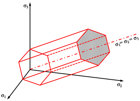
Figure 9. Tresca failure criterion (according to Nova, 2005).

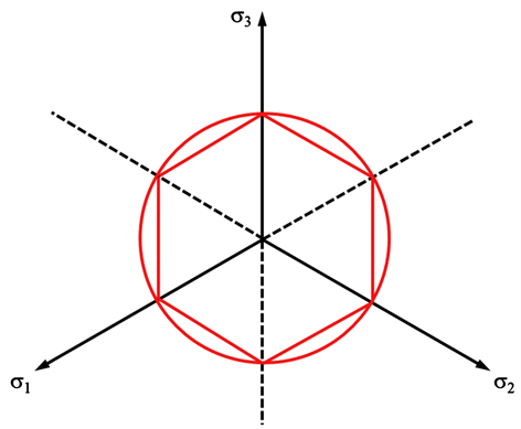
Figure 10. Deviatoric plane section of the tresca and von mises failure criteria (based on Nova, 2005).

${\sigma }_1^2+{\sigma }_2^2+{\sigma }_3^2-{\sigma }_1{\sigma }_2-{\sigma }_1{\sigma }_3-{\sigma }_2{\sigma }_3-{\sigma }_{rupt}^2\le 0$ (57)

The Mohr-Coulomb failure criterion is widely employed in geotechnical calculations. It postulates a linear relationship between the maximum shear stress and the normal stress. On a Mohr diagram, this is akin to considering that the intrinsic curve (i.e., the envelope of the Mohr circles associated with failure) forms a straight line (refer to Figure 11).

The Mohr-Coulomb criterion can take various forms based on soil characteristics and the speed of applied loading. In saturated soils, two types of behavior are distinguished: drained and undrained. Drained long-term behavior occurs when the applied load meets one of the following conditions:

• It progresses sufficiently slowly, considering the soil permeability and drainage path length, so as not to induce significant interstitial overpressure at any point.

• It has persisted long enough for any potential interstitial overpressures to dissipate by the time soil behavior is assessed.

Short-term undrained calculations correspond to situations immediately following the rapid application of load, associated with undrained characteristics. Table 2 compiles the main failure criteria and the mechanical tests required for their estimation.

In the subsequent part of the paper, a long-term drained behavior is taken into account. In this type of scenario, it is assumed that the loads are entirely transferred to the soil skeleton, leading to the utilization of effective quantities. The Mohr-Coulomb criterion associated with this behavior is expressed by Equation (58).

${\tau }_{rupt}=C^{\prime }+{\sigma }^{\prime }\tan {\varphi }^{\prime }$ (58)

Table 2. Selection of failure criterion (based on Magnan, 1991).

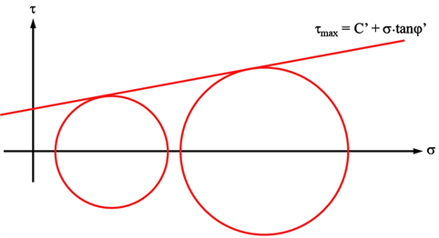
Figure 11. Mohr-coulomb line.

where $C^{\prime }$ is the effective cohesion, ${\varphi }^{\prime }$ is the internal friction angle, and ${\sigma }^{\prime }$ is the effective normal stress.

In terms of principal stresses, the failure condition according to the Mohr-Coulomb criterion is met when one of the following relationships is satisfied with equality (Equation (59)):

$\left|{\sigma }_i-{\sigma }_j\right|-\left({{\sigma }^{\prime }}_i-{{\sigma }^{\prime }}_j\right)\sin {\varphi }^{\prime }-2C^{\prime }\cos {\varphi }^{\prime }\le 0$ (59)

where the indices i and j take the values 1, 2, and 3 through permutation.

When the equations Equation (59) are satisfied with equality, they provide the equations for six planes that define a volume in the space of principal stresses. This volume takes the form of a pyramid with an axis such that ${{\sigma }^{\prime }}_1={{\sigma }^{\prime }}_2={{\sigma }^{\prime }}_3$ , and its cross sections are irregular hexagons (see Figure 12). Since soil cannot withstand tensile stresses, the three relationships in Equation (60) are also to be considered.

${{\sigma }^{\prime }}_i\ge 0$ (60)

The gradient of the plasticity function obtained from the Mohr-Coulomb criterion is not defined on the edges of the pyramid. Therefore, Drucker and Prager (1952) [42] proposed the following formulation (Equation (61)):

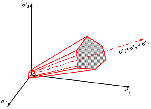
Figure 12. Mohr-Coulomb Failure Criterion (based on Nova, 2005).

${{\sigma }^{\prime }}_1^2+{{\sigma }^{\prime }}_2^2+{{\sigma }^{\prime }}_3^2-{{\sigma }^{\prime }}_1{{\sigma }^{\prime }}_2-{{\sigma }^{\prime }}_1{{\sigma }^{\prime }}_3-{{\sigma }^{\prime }}_2{{\sigma }^{\prime }}_3-{\left(\mu \left({{\sigma }^{\prime }}_1+{{\sigma }^{\prime }}_2+{{\sigma }^{\prime }}_3\right)+K\right)}^2=0$ (61)

where $\mu$ and K can be chosen in such a way that the cone defined by this equation encompasses the Mohr-Coulomb pyramid (see Figure 13).

The Drucker postulate of normality connects the stress state at the moment of plasticity to plastic deformations. It can be expressed as (Equation (62)):

$d{\epsilon }_{ij}^p=\Lambda \frac{\partial f}{\partial {\sigma }_{ij}}$ (62)

If Equation (62) is satisfied, it is said that the material is standard and that the flow law is associated with it. For soils, this equation is not always valid, which is why the notion of dilatancy is sometimes introduced.

With the Drucker and Prager failure criterion, the principal components of the plastic strain increment tensor are given by (Equation (63)):

$\left[\begin{array}{c}d{\epsilon }_1^p\\ d{\epsilon }_2^p\\ d{\epsilon }_3^p\end{array}\right]=\Lambda \cdot \left[\begin{array}{c}3{{\sigma }^{\prime }}_1-3\left(1+2\mu \right)p^{\prime }-2K\\ 3{{\sigma }^{\prime }}_2-3\left(1+2\mu \right)p^{\prime }-2K\\ 3{{\sigma }^{\prime }}_3-3\left(1+2\mu \right)p^{\prime }-2K\end{array}\right]$ (63)

2.3. Stability Analysis

Stability analysis of a slope, whether it pertains to natural terrain or an artificial embankment, aims to address two fundamental questions:

What is the likelihood of a landslide occurrence?

If a landslide does occur, what is the geometry of the failure surface?

The answers to these questions, based on the specific context, are crucial in identifying potential sliding scenarios and deriving conclusions to ensure the safety of both individuals and structures. Conducting stability analyses for embankments presents a complex challenge due to the multitude of influencing

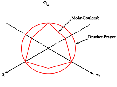
Figure 13. Deviatoric plane section of mohr-coulomb and drucker-prager failure criteria (adapted from Nova, 2005).

factors, including topography, hydraulic conditions, human activities (such as construction projects or dam drainage), and geological characteristics. Additionally, the mechanical properties of soils often exhibit heterogeneity, anisotropy, and discontinuities. Generally, three primary types of instabilities are recognized: slides involving distinct failure surfaces (often circular in shape), mudflows, and rockfalls. For the scope of this study, we will focus solely on the first type of instability.

A safety factor, denoted as F, serves as an indicator of the risk associated with potential slope failure. It is influenced by the selected calculation method, the stress state within the slope, the properties of the medium, and the geometry of the failure surface. Two distinct definitions are commonly used [43] [44] .

According to the first definition, the safety factor is the value by which the soil’s strength must be divided to initiate a failure. This factor is represented as F₁. This definition is widely adopted and is utilized in equilibrium-based methods, as well as in the subsequently described SSRM and GIM methods.

The second, more physically grounded definition, characterizes the safety factor as the ratio between resisting forces and driving forces (Equation (64)), denoted as F₂.

$F_2=\frac{{\displaystyle {\int }_s{\tau }_{rupt}\text{d}s}}{{\displaystyle {\int }_s\tau \text{d}s}}$ (64)

In theory, if F is less than 1, the slope is considered unstable. Conversely, if F is greater than 1, the slope is deemed stable. In practical terms, to account for uncertainties stemming from calculations or the determination of site characteristics, a safety factor is introduced according to Duncan (1996) [45] . Broadly, the following guidelines are followed:

• If $F<1$ , there is a hazard;

• If $1\le F<1.25$ , safety is subject to question;

• If $1.25\le F<1.4$ , safety might be judged acceptable if the potential consequences of a slope failure are minimal;

• If $F\ge 1.4$ , safety is considered satisfactory.

The specified ranges of values can be adjusted depending on the potential impact of a slope failure.

2.3.2. Determination of Critical Failure Surface, 2D or 3D Analysis

The systematic quest for the critical failure surface entails, in its initial phase, delineating a set of potential failure surfaces: one might opt, for instance, to confine consideration to planar or circular failure surfaces (this selection should be informed by on-site observations). Subsequently, the safety factor is computed for each of these surfaces. The critical failure surface is the one linked to the smallest safety factor. This straightforward technique yields satisfactory outcomes in the majority of cases; however, it necessitates testing a considerable number of failure surfaces, a process that can be laborious. Moreover, it mandates restricting the analysis to geometrically uncomplicated failure surfaces.

Due to these considerations, algorithms designed to identify critical failure surfaces have been introduced, and these include contributions by Baker (1980), Celestino & Duncan (1981), Greco & Gulla (1985), Nguyen (1985), Li & White (1987), Chen (1992), Greco (1996), Hussein et al. (2001), and Cheng (2003), among others [46] - [54] .

Presently, most stability assessments are conducted within a 2D framework; however, as computational capabilities continue to advance, the adoption of a three-dimensional approach is progressively gaining traction. Generally, safety factors calculated in 2D are marginally lower than those computed in 3D, as 2D analysis focuses on the cross-section of a slope that is the least stable.

2.3.3. Key Limit Equilibrium Methods

Currently, limit equilibrium methods remain the most widely employed techniques for conducting stability analyses. These methods involve partitioning the soil into sufficiently narrow slices such that their bases can be approximated as straight segments. The next step is to formulate equilibrium equations for forces and/or moments. Various adaptations have emerged based on the assumptions about forces between slices and the chosen equilibrium equations (Table 3). These adaptations typically yield reasonably consistent outcomes, with discrepancies in computed F values often remaining below 6%, as reported by Duncan (1996) [45] .

The benchmark limit equilibrium methods are the formulations proposed by Fellenius (1927) [55] and Bishop (1955) [56] . Figure 14 illustrates the division of a potentially unstable slope. The horizontal equilibrium for slice i can be expressed as (Equation (65)):

$\text{d}{H}_i-{\sigma }_i\tan {\alpha }_i\text{d}x+{\tau }_i\text{d}x=0$ (65)

Here, $H_i$ represents the horizontal force component between two slices, ${\sigma }_i$ and ${\tau }_i$ denote the normal and tangential stresses on the potential failure surface

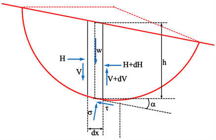
Figure 14. Circular failure analysis using bishop and fellenius approaches.

Table 3. Key limit equilibrium methods.

at the level of slice i and ${\alpha }_i$ signifies the angle formed between the base of slice i and the horizontal (Figure 14).

The vertical equilibrium for slice i can be described by (Equation (66)):

$\text{d}{V}_i-{\gamma }_i{h}_i\text{d}x+{\sigma }_i\text{d}x+{\tau }_i\tan {\alpha }_i\text{d}x=0$ (66)

In this equation, $V_i$ indicates the vertical force component between two slices, and ${\gamma }_i$ represents the weight of slice i.

In Fellenius’s method (1927), an assumption is made that both $\text{d}{H}_i$ and $\text{d}{V}_i$ are equal to zero, leading to the estimation of normal stresses using (Equation (67)):

${\sigma }_i=\gamma h_i{\cos }^2{\alpha }_i$ (67)

By utilizing the global definition of the safety factor, Equation (68) is obtained.

In Bishop’s method (1955), the assumption $\text{d}{V}_i=0$ is employed. By considering the global definition of the safety factor, is derived: ${\sigma }_i={\gamma }_i{h}_i-{\tau }_i\left(F_{\text{Bish}}\right)\tan {\alpha }_i$ This yields a relationship of the form: $F_{\text{Bish}}=f\left(F_{\text{Bish}}\right)$ (Equation (69)). The safety factor is determined using an iterative process known as the fixed-point method. For instance, Alexis (1987) [63] applied this method to study the stability of sediment ponds and channels in the Lorient harbor.

$F_{\text{Fel}}=\frac{{\displaystyle \underset{i=1}{\overset{n}{\sum }}}\left(C^{\prime }+\left(\gamma h_i{\cos }^2{\alpha }_i-u_i\right)\tan {\phi }^{\prime }\right)\frac{1}{\cos {\alpha }_i}}{{\displaystyle \underset{i=1}{\overset{n}{\sum }}}\gamma h_i\sin {\alpha }_i}$ (68)

$F_{\text{Bish}}=\frac{{\displaystyle \underset{i=1}{\overset{n}{\sum }}}\left(C^{\prime }+\left(\gamma h_i-\left(\frac{C^{\prime }}{F_{\text{Bish}}}+{\sigma }^{\prime }\frac{\tan {\phi }^{\prime }}{F_{\text{Bish}}}\right)\tan {\alpha }_i-u_i\right)\tan {\phi }^{\prime }\right)\frac{1}{\cos {\alpha }_i}}{{\displaystyle \underset{i=1}{\overset{n}{\sum }}}\gamma h_i\sin {\alpha }_i}$ (69)

In certain slope scenarios, failure can occur approximately parallel to the slope surface. The calculation model utilized assumes an infinite soil with the water table parallel to the slope surface (see Figure 15). Considering the assumption of an infinite slope, the vertical forces exerted on the block’s sides can be considered negligible ( $V=0$ ). Assuming equilibrium of horizontal forces and pressures on each side of the block and stipulating the sum of applied forces is zero, the normal and tangential reactions at the base of the block can be calculated. Thus, employing the Mohr-Coulomb criterion and accounting for long-term drained behavior, the expression for the safety factor can be deduced as follows (Equation (70)):

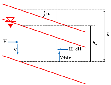
Figure 15. Failure plane.

$F=\frac{2}{\sin \left(2\alpha \right)}\frac{C^{\prime }}{g\rho }+\frac{\left(\rho h-{\rho }_w{h}_w\right)\tan {\phi }^{\prime }}{\rho h\tan \alpha }$ (70)

Two primary factors contribute to the prevalence of limit equilibrium methods:

• They are straightforward, familiar, and comprehensible to all stakeholders in the field;

• They rely on a limited set of parameters, avoiding the need to parameterize soil behavior laws, for instance.

However, these methods do have significant limitations. They do not incorporate soil behavior, struggle to accurately address complex scenarios (such as construction stages, dynamic loads, hydro-mechanical coupling, etc.), and assume constant safety factors along the failure surface (utilizing the global definition of the safety factor F₁).

2.3.4. Finite Element Methods (FEM)

With the continuous improvement of computational capabilities, the utilization of finite element methods for stability analysis is progressively expanding. This approach offers several distinct advantages. It allows for the highly realistic modeling of slopes, encompassing intricate geometries, loading sequences, reinforcement arrangements, hydro-mechanical coupling, complex soil behavior laws, and more. Additionally, it provides insights into soil deformations, and transitioning from 2D to 3D is more seamless compared to limit equilibrium methods.

Three stability analysis techniques based on FEM stand out. The Shear Strength Reduction Method (SSRM), introduced by Zienkiewicz et al. in 1975 and later explored by various researchers including Naylor (1981), Donald and Giam (1988), Matsui and San (1992), Ugai and Leshchinsky (1995), Dawson et al. (1999), Griffiths and Lane (1999), Jeremić (2000), and Zheng et al. (2005), among others [64] - [72] . The fundamental principle involves conducting an initial calculation under “normal” conditions. Subsequently, the soil’s resistance characteristics are systematically reduced (employing the first definition of the global factor of safety) until the calculation diverges. The factor of safety is then determined as the last F1 value at which the calculation converged. This technique rests on the hypothesis that calculation divergence signifies slope instability. In essence, the SSRM posits that calculation divergence occurs when, prompted by a rapid increase in displacements due to slope failure, the equilibrium equations can no longer be satisfied. The use of a criterion based on a “non-solution” approach is unconventional and can present certain challenges. Firstly, accurately pinpointing the “non-convergence” point is quite intricate. Furthermore, achieving a high level of precision in determining whether divergence indeed results solely from mass instability necessitates meticulous numerical analysis. Lastly, the very definition of the factor of safety presupposes that its constancy along the rupture surface is maintained, a notion that deviates from reality. Nevertheless, the principal merit of this method lies in the fact that it requires no a priori assumptions regarding the geometry of the failing mass; the rupture surface emerges automatically, corresponding to the region where deformations attain their maximum.

The Gravity Increase Method (GIM) shares a comparable principle with SSRM, except that instead of systematically diminishing the soil’s resistance attributes until instability is triggered, the impact of gravity is intensified. Consequently, the factor of safety in GIM is established as the ratio between the gravity value at failure and the standard gravity value. GIM is particularly applicable for assessing slope stability during the construction of structures.

The third FEM-based method involves computing the factor of safety for prospective rupture surfaces using Equation (64). Within this framework, the factor of safety is not uniformly constant along the rupture surfaces. A distinct advantage, compared to SSRM or GIM, is the avoidance of a criterion tied to calculation divergence. Nonetheless, determining the critical rupture surface necessitates a comprehensive search. This approach has been explored by researchers including Yamagami and Ueta (1988), Zou and Williams (1995), Farias and Naylor (1998), Wang (1999), and Thiébot (2004), among others [73] [74] [75] [76] [77] .

2.4. Soils Transport Modeling in Unstable Terrains

To effectively incorporate a soil/consolidation model into a hydro-sedimentary computational framework, it’s imperative to consider how:

Various water/sediment mixtures are characterized (diluted suspension, slurry, cohesive bed), processes such as transport, deposition, erosion, and more are simulated. The objective of this section is to delineate classical modeling strategies. Depending on the specific context, there are several conceivable levels of modeling. The three-dimensional approach, being the most comprehensive, allows for the calculation of parameter evolution along the vertical axis and across the horizontal axes (Blumberg and Mellor, 1987; Nicholson and O’Connor, 1986; Lang et al., 1989; Lazure and Jegou, 1998; Cancino and Neves, 1998; Le Normant, 2000; Phan, 2002) [28] [78] - [83] . However, this approach requires substantial computational resources. The vertical two-dimensional approach (2DV) permits parameter evolution calculation along the longitudinal and vertical axes, but not across transverse sections (Boerick and Hogan, 1977; Rodger and Odd, 1985; Li, 1994; Li et al., 1994; Sheng and Villaret, 1989; Brun-Cottan et al., 2000) [84] [85] [86] [87] [88] . The horizontal two-dimensional approach (2DH) involves vertical integration of variables and is commonly employed in sedimentology. It provides insight into the evolution of parameters along the estuary’s longitudinal axis and across transverse sections but does not account for vertical variations (Cole and Miles, 1983; Teisson and Latteux, 1986; Odd and Cooper, 1989; Falconer and Owen, 1990; Guillou and N’Guyen, 1999; Malchereck, 2000) [89] - [94] . This approach is well-suited for well-mixed estuaries. The one-dimensional approach involves integrating variables along the vertical and across transverse sections, providing a depiction of phenomena along the estuary’s longitudinal axis (Odd and Owen, 1972; Uncles and Stephens, 1989; Le Hir and Karlikow, 1991) [95] [96] [97] .

2.4.1. Hydrodynamic Calculation in Unstable Terrains

The Navier-Stokes equations serve as the fundamental basis for hydrodynamic calculations. They encompass a continuity equation (or mass conservation equation) and a vectorial equation for the transport of momentum.

In the context of assuming a nearly incompressible fluid (Boussinesq Hypothesis), employing the ${\beta }^3$ plane approximation (Pedlosky, 1987) [98] , and considering that the water depth is small in relation to the horizontal extent of the domain, the three-dimensional form of the equations governing shallow water flow takes the following shape:

$\{\begin{array}{l}\frac{\partial u_i}{\partial t}+\frac{\partial u_i}{\partial x_j}=f_i-\frac{1}{{\rho }_r}\frac{\partial p}{\partial x_i}+\frac{1}{{\rho }_r}\frac{\partial {\tau }_{ij}}{\partial x_j}\\ \frac{\partial p}{\partial z}=-{\rho }_w\cdot g\\ \frac{\partial u_j}{\partial x_j}=0\end{array}$ (71)

where u represents the flow velocity, f denotes the Coriolis force, p stands for the pressure at depth z, ${\rho }_r$ signifies the reference mass density of water, and ${\tau }_{ij}$ represents the stress tensor encompassing both viscous and turbulent effects.

The Saint-Venant equations emerge through the vertical integration of Equation (71) (as seen in Guillou, 1996 [99] and similar sources). These equations presuppose minimal vertical variations in velocity. Under these assumptions, the model is simplified to a two-dimensional framework with the variables being the flow velocities along the x and y axes, denoted as U and V respectively, alongside the water depths, represented as H.

$\{\begin{array}{l}\frac{\partial \eta }{\partial t}+\frac{\partial H{U}_i}{\partial x_i}=0\\ \underset{\text{I}}{\underset{︸}{\frac{\partial H{U}_i}{\partial t}+\frac{\partial U_{k}H{U}_i}{\partial x_k}}}=\underset{\text{II}}{\underset{︸}{F_i}}-\underset{\text{III}}{\underset{︸}{gH\frac{\partial \eta }{\partial x_i}}}-\underset{\text{IV}}{\underset{︸}{g\frac{\partial H\langle \sigma \rangle }{\partial x_i}}}+\underset{\text{V}}{\underset{︸}{\frac{{\tau }_{si}-{\tau }_{bi}}{{\rho }_r}}}+\underset{\text{VI}}{\underset{︸}{\frac{\partial H\langle {\tau }_{ik}\rangle }{\partial x_k}}}-\underset{\text{VII}}{\underset{︸}{\frac{\partial H\langle {u^{\prime }}_i{u^{\prime }}_k\rangle }{\partial x_k}}}\end{array}$ (72)

where $\eta$ represents the elevation (where the water height H is equal to $h+\eta$ , with h being the seabed elevation relative to a reference level), $F_i$ denotes the Coriolis effects, g signifies the gravitational acceleration, $\langle f\rangle =$ Equation (73), Equation (74) stands for the buoyancy term, ${\tau }_{si}$ is the wind stress applied to the free surface, ${\tau }_{bi}$ represents the shear stress at the seabed (friction), and ${u^{\prime }}_i$ is the dimensionless flow velocity.

$\langle f\rangle =\frac{1}{H}{\displaystyle \underset{-h}{\overset{\eta }{\int }}f\text{d}z}$ (73)

$\sigma ={\displaystyle \underset{z}{\overset{\eta }{\int }}}\frac{\left|{\rho }_w-{\rho }_r\right|}{{\rho }_r}\text{d}{z}^{\prime }$ (74)

In Equation (72), the Roman numerals I to VI correspondingly indicate inertial effects, Coriolis effects, the influence of pressure gradient, the buoyancy term, effects of surface wind and seabed friction, as well as the viscous effects resulting from turbulence. Term VII introduces dispersion, reflecting the impact of the vertical velocity profile on the average flow.

2.4.2. Conventional Approach to Modeling Soils Transport in Unstable Terrains

Most soil transport models (such as SIAM, MIKE, TELEMAC, as well as academic models) are built upon a simplifying assumption that sediment particles move at the same velocity as the fluid particles, except for their settling velocity (Li et al., 1994; Brenon, 1997; Le Normant, 2000; Phan, 2002; Tattersall et al., 2003; Lumborg and Morten, 2005; Markofsky and Ditschke, 2007, …) [28] [83] [100] [101] [102] [103] . This assumption is commonly referred to as the “passive scalar” hypothesis. Under this assumption, the impact of sediment on the flow is neglected, and the seabed is conceptually defined at the upper level of sediment deposits (slurry and cohesive bed). These deposits form a sediment reservoir that undergoes emptying or filling through processes of erosion and deposition (Figure 16).

A more recent and evolving biphasic approach involves considering an interaction between a solid phase and a fluid phase. In this model, there is no need to introduce a fictitious bed, as it is naturally encompassed within the computational domain. Several attempts have been made using this approach (Le Hir, 1994; Vilaret et al., 1996; Greimann et al., 1999; Barbry, 2000; Barbry et al., 2000; Hsu et al., 2003; Jiang et al., 2004; Amoudry et al., 2005; Chauchat, 2007) [104] - [112] .

In the subsequent stages of this article, we confine our analysis to the conventional single-phase approach.

2.4.3. Transport of Soils in Diluted Suspension

Under the assumption of the passive scalar, the transport of soil is determined by an equation such as Equation (75). However, this holds true only when soil

Figure 16. Conventional single-phase approach.

concentrations in the diluted suspension (denoted as Cs) remain low (below a few g/l). Beyond these concentration levels:

• Particle interactions can no longer be ignored, as they influence the rheological behavior of the suspension (which can no longer be assumed as Newtonian), the mode of sediment transport, and the mechanism governing sediment settling;

• The volume occupied by sediment can no longer be considered negligible.

$\begin{array}{l}\frac{\partial C_s}{\partial t}+u\frac{\partial C_s}{\partial x}+v\frac{\partial C_s}{\partial y}+w\frac{\partial C_s}{\partial z}+\frac{\partial W_s{C}_s}{\partial z}\\ =\frac{\partial }{\partial x}\left(K_x\frac{\partial C_s}{\partial x}\right)+\frac{\partial }{\partial y}\left(K_y\frac{\partial C_s}{\partial y}\right)+\frac{\partial }{\partial z}\left(K_z\frac{\partial C_s}{\partial z}\right)+\frac{F_e-F_d}{H}+S\end{array}$ (75)

where C_s represents the sediment concentration in the diluted suspension, u, v, and w denote fluid flow velocities, W_s indicates the sediment settling velocity, F_e and F_d stand for erosion and deposition fluxes, H signifies the water depth, K_x, K_y, and K_z are terms for turbulent diffusion, and S represents a source term.

In the diluted suspension, the sediment settling velocity W_s can be correlated with the concentration C_s, temperature, turbulence, or salinity to account for effects induced by flocculation.

While slurry constitutes a suspension, attempting to simulate its movements using an equation like Equation (75) is unfeasible due to the concentrations typically present in slurry, which render the passive scalar assumption inapplicable. Consequently, it is commonly regarded as part of the seabed.

In the classical approach, the interactions between the bed and the diluted suspension are managed through the utilization of deposition and erosion fluxes. These are typically derived using the formulations introduced by Krone (1962) and Partheniades (1962) [113] [114] .

Krone’s deposition law (1962) [113] (Equation (76)) stipulates that deposition occurs only when the frictional stress at the bottom is lower than a critical stress denoted as ${\tau }_{0d}$ . The commonly adopted value for ${\tau }_{0d}$ is approximately 0.1 N∙m².

$F_d=\{\begin{array}{ll}{W}_s{C}_s\left(1-\frac{{\tau }_b}{{\tau }_{cd}}\right)\hfill & \mathrm{<mtext>\; \hspace{0.17em}\; </mtext>\; <mtext>\; \hspace{0.17em}\; </mtext>}\text{if}{\tau }_b<{\tau }_{cd}\hfill \\ 0\hfill & \mathrm{<mtext>\; \hspace{0.17em}\; </mtext>\; <mtext>\; \hspace{0.17em}\; </mtext>}\text{if}{\tau }_b\ge {\tau }_{cd}\hfill \end{array}$ (76)

Erosion takes place when the bottom friction stress exceeds a critical stress indicated as ${\tau }_{0e}$ . This critical stress marks the point at which the stress caused by the flow over the bed becomes potent enough to overcome the cohesive and gravitational forces that anchor the particles to the bed (Partheniades, 1962) [114] . The erosion law formulated by Partheniades (1962) is outlined in Equation (77).

$F_e=\{\begin{array}{ll}M\left(\frac{{\tau }_b-{\tau }_{ce}}{{\tau }_{ce}}\right)\hfill & \mathrm{<mtext>\; \hspace{0.17em}\; </mtext>\; <mtext>\; \hspace{0.17em}\; </mtext>}\text{if}{\tau }_b>{\tau }_{ce}\hfill \\ 0\hfill & \mathrm{<mtext>\; \hspace{0.17em}\; </mtext>\; <mtext>\; \hspace{0.17em}\; </mtext>}\text{if}{\tau }_b\le {\tau }_{ce}\hfill \end{array}$ (77)

where M represents the Partheniades constant and ${\tau }_{0e}$ is the critical shear stress at the bed for erosion. The critical erosion stress is dependent on the bed’s consolidation level. Notably, freshly deposited mud is more easily resuspended than consolidated mud. Metha (1991) [115] classifies three distinct erosion types:

• Entrainment or resuspension, occurring in fluid mud with low rigidity. In such scenarios, even very minimal stress at the bottom can suffice to resuspend sediment ( ${\tau }_{0e}<0.1\text{N}\cdot {\text{m}}^{-\text{2}}$ ).

• Floc detachment, the most frequently observed mechanism. For this kind of erosion to take place, bed friction needs to be sufficient to overcome electrochemical forces binding the flocs ( $0.1\text{N}\cdot {\text{m}}^{-\text{2}}<{\tau }_{0e}<1\text{N}\cdot {\text{m}}^{-\text{2}}$ ).

• Vase block detachment in consolidated mud, under significant bottom stress ( ${\tau }_{0e}>1$ N∙m⁻²).

Depending on the hydro-sedimentary characteristics of the site under modeling and the intended simulation type, several strategies can be considered to address bed evolution due to hindered settling and consolidation effects. Below are descriptions of the most prevalent approaches.

The simplest method involves considering a uniform bed with a set concentration (e.g., Tattersall et al., 2003) [101] . Conventionally, the bed is portrayed as layers with varying thicknesses and fixed concentrations.

Precisely defining the concentration range of the layers comprising the bed is crucial as it directly impacts the way exchanges unfold between the diluted suspension and the bed. Typically, the minimum concentration value of muddy deposits (i.e., the uppermost layer’s concentration) is chosen to be around 100 g/l (Teisson, 1993; Guesmia, 2001; Lumborg and Windelin, 2003) [116] [117] [118] . This value corresponds to a standard concentration for slurry.

When assuming that slurry is integral to the bed (Li, 1994, or Petersen and Vested, 2002) [86] [119] :

• This involves considering it to be immobile, i.e., it doesn’t move on the bed due to currents or bed slope.

• This approach facilitates a “reasonable” concentration transition between the diluted suspension and the bed.

Several techniques for managing sediment distribution among layers are presented below.

The empirical multilayer model developed by Teisson (1991, 1993) [116] [120] is incorporated within the TELEMAC system. It involves representing the bed with layers, each possessing fixed concentrations and residence times. During deposition, sediment fills the uppermost layer, increasing its thickness correspondingly. The time sediment spends in the layer is logged; if it exceeds the layer’s associated residence time (assuming sediment hasn’t been resuspended by erosion), all sediment within that layer is transferred to the underlying, more concentrated layer. This process continues for all layers. Residence times T_i and layer concentrations C_i are derived by discretizing a compaction curve using a piecewise function (Figure 17).

Figure 17. Determining parameters for teisson’s empirical model (1993).

The second model available in TELEMAC was developed by Le Normant (2000) [28] . This model focuses on pure consolidation (i.e., hindered settling effects in the mud layer are not considered). It applies to beds where the concentration is equal to or greater than Ct (which is approximately 200 g/l according to Sanchez, 1992, or Thiébot, 2006c) [121] [122] .

Le Normant’s model (2000) [28] involves discretizing the Gibson equation Equation (40) in an implicit form. This results in a system of equations that utilizes a tridiagonal matrix. Thus, the double-sweep method (or Thomas algorithm) can be used to determine the indices of voids at each node of a mesh defined between the ZF and ZR levels (Figure 16). To manage data effectively, a maximum number of nodes (or planes), nbmax, is defined. A layer referred to as the “fresh deposit layer” acts as the transition between the diluted suspension and the bed (the cohesive bed). This layer has a fixed concentration denoted as Conc0. When its thickness exceeds a certain value, Epai0, the sediment it contains is transferred to the cohesive bed. This sediment transfer is accounted for either by introducing a new plane if the plane count is below nbmax, or by re-discretizing the cohesive bed if the maximum plane count has been reached.

The empirical compaction model integrated into SIAM is based on the work of Le Hir (1989) [123] . It has been expanded to cover mixed sediments (sandy-silty) by Waeles (2005) [124] . This model involves determining the relative concentration of mud $C_{\text{mud},\text{rel}}$ (Equation (78)) for each discretized bed layer using a differential equation (Equation (79)):

$C_{\text{mud},\text{rel}}=\frac{m_{\text{mud}}}{V_{\text{total}}-V_{\text{sand}}}$ (78)

$\frac{\partial C_{\text{mud},\text{rel}}}{\partial t}=A_1\text{exp}\left(-A_2{C}_{\text{mud},\text{rel}}\right)\left[C_{\text{mud},\text{rel},\text{max}}\left(1+A_3{\displaystyle \underset{z}{\overset{h}{\int }}}\left(\rho -{\rho }_w\right)\text{d}z\right)-C_{\text{mud},\text{rel}}\right]$ (79)

where $A_i$ are empirical constants, and Equation (80) is the maximum value that $C_{\text{mud},\text{rel}}$ can reach, considering the depth of the layer relative to the upper part of the deposit.

$C_{\text{mud},\text{rel},\text{max}}\left(1+A_3{\displaystyle \underset{z}{\overset{h}{\int }}}\left(\rho -{\rho }_w\right)\text{d}z\right)\mathrm{<mtext>\; \hspace{0.17em}\; </mtext>\; <mtext>\; \hspace{0.17em}\; </mtext>\; <mtext>\; \hspace{0.17em}\; </mtext>\; <mtext>\; \hspace{0.17em}\; </mtext>\; <mtext>\; \hspace{0.17em}\; </mtext>\; <mtext>\; \hspace{0.17em}\; </mtext>}\text{maximumvalueof}{C}_{\text{mud},\text{rel}}$ (80)

3. Conclusions

This comprehensive exploration of geotechnical engineering has illuminated various facets crucial to understanding and managing unstable terrains. We have traversed the intricate terrain of cohesive sediments, uncovering their unique physicochemical properties, including cohesion and specific surface area. This foundational knowledge is fundamental to any geotechnical endeavor, as it forms the bedrock upon which subsequent analyses are built.

The temporal evolution of deposit concentration and average bed concentration in unstable terrains has been scrutinized, shedding light on the dynamic processes that shape these environments. Understanding settling behavior, from the principles of Stokes’ settling velocity to hindered settling via Richardson and Zaki’s law, is paramount in predicting sediment behavior in real-world scenarios.

Our journey has taken us through key sedimentation theories, notably Kynch’s theory, and geotechnical consolidation theories, including Terzaghi’s consolidation equation and Gibson’s theory. By interrelating these theories and principles, we have provided a holistic view of managing unstable terrains. This interconnected perspective empowers geotechnical engineers to make informed decisions and design resilient structures in a world of shifting soils.

Yet, challenges persist, particularly in the experimental determination of constitutive relationships. We’ve addressed these challenges and offered alternative simplification methods to navigate these complexities efficiently.

Furthermore, we’ve delved into the numerical methods essential for solving the nonlinear partial differential equations that govern soil behavior. These methods, ranging from finite difference to finite element techniques, are the backbone of modern geotechnical analysis. We’ve acknowledged the challenges, including deformable meshes and discontinuous concentration profiles, and emphasized the need for numerical frameworks.

The paper’s exploration of rheological analysis has uncovered the complex material flow behaviors of suspensions and muddy soils. We’ve navigated the diverse rheological behavior models and explored the unique properties of water and cohesive sediment mixtures, from viscoelasticity to yield stress. This knowledge equips geotechnical engineers with the tools to predict and manage the flow of materials in various contexts.

Fundamental geotechnical calculations, constitutive laws, and failure criteria have been presented, showcasing their relevance in geotechnical engineering applications. These foundational principles underpin our ability to analyze and design structures that withstand the challenges posed by unstable terrains.

In essence, this paper has offered a multidimensional perspective on geotechnical engineering. It has provided valuable insights into soil properties, consolidation processes, numerical methodologies, rheological analyses, and slope stability assessments. Armed with this knowledge, geotechnical professionals are better prepared to tackle the complexities and uncertainties inherent in their field, ultimately contributing to safer and more resilient infrastructure worldwide. As we look to the future, the continued advancement of geotechnical science and engineering promises even greater capabilities and solutions for managing unstable terrains and ensuring the stability and safety of our built environment.

Acknowledgements

Authors gratefully acknowledge financial support for this work from National Natural Science Foundation of China: Major building and bridge structures and Earthquake Disaster Integration (91315301).

Data Availability Statement

Some or all data, models, or code that support the findings of this study are available from the corresponding author upon reasonable request.

Conflicts of Interest

The authors declare no conflicts of interest regarding the publication of this paper.

References

[1]	Buffle, J. and Chalmers, R.A. (1988) Complexation Reactions in Aquatic Systems: An Analytical Approach. Ellis Horwood Series in Analytical Chemistry, John Wiley and Sons Inc., New York. https://www.osti.gov/biblio/6446347
[2]	Been, K. and Sills, G.C. (1981) Self-Weight Consolidation of Soft Soils: An Experimental and Theoretical Study. Geotechnique, 31, 519-535. https://doi.org/10.1680/geot.1981.31.4.519
[3]	Alexis, A., Bassoullet, P., Le Hir, P. and Teisson, C. (1992) Consolidation of Soft Marine Soils: Unifying Theories, Numerical Modelling and in situ Experiments. Coastal Engineering, 2949-2961. https://doi.org/10.1061/9780872629332.225
[4]	Gallois, S. (1995) Modélisation de la sédimentation-consolidation et expérimentations sur les vases estuariennes, Nantes. https://www.theses.fr/1995NANT2071
[5]	Masutti, F. (2001) étude expérimentale de la sédimentation-consolidation et de l’acquisition de résistance d’un sol fin, Institut National Polytechnique de Lorraine. https://hal.univ-lorraine.fr/tel-01750328
[6]	Alexis, A., Lebras, G. and Thomas, P. (2004) Experimental Bench for Study of Settling-Consolidation Soil Formation. Geotechnical Testing Journal, 27, 557-567. https://doi.org/10.1520/GTJ11582
[7]	Pham Van Bang, D., Lefrançois, E., Sergent, P. and Bertrand, F. (2006) Approche expérimentale par IRM et modélisation de la sedimentation et de la consolidation de la vase. IXèmes Journées Nationales Génie Civil—Génie Côtier, Brest, 12-14 Septembre 2006, 409-417. https://doi.org/10.5150/jngcgc.2006.039-P
[8]	Migniot, C. (1968) Etude des propriétés physiques de différents sédiments très fins et de leur comportement sous des actions hydrodynamiques. La Houille Blanche, 54, 591-620. https://doi.org/10.1051/lhb/1968041
[9]	Winterwerp, J.C. and Van Kesteren, W.G.M. (2004) Introduction to the Physics of Cohesive Sediment Dynamics in the Marine Environment. Elsevier Science, Amsterdam.
[10]	Alves, M.C.M. (1992) Comportamento de sedimentação e adensamento de uma lama vermelha. Ph.D. Thesis, Pontifcia Universidade Católica do Rio de Janeiro, Rio de Janeiro.
[11]	Hayter, E.J. (1986) Estuarial Sediment Bed Model. Estuarine Cohesive Sediment Dynamics, 14. https://doi.org/10.1029/LN014p0326
[12]	Stokes, G.G., et al. (1851) On the Effect of the Internal Friction of Fluids on the Motion of Pendulums. In: Stokes, G.G., Ed., Mathematical and Physical Papers, Cambridge University Press, Cambridge, 1-10.
[13]	Oseen, C.W. (1927) Neuere methoden und ergebnisse in der hydrodynamic. Monatshefte für Mathematik und Physik, 35, A67-A68.
[14]	Richarson, J.F. and Zaki, W.N. (1954) Sedimentation and Fluidisation, Part 1. Chemical Engineering Research and Design, 75, S82-S100.
[15]	Kynch, G.J. (1952) A Theory of Sedimentation. Transactions of the Faraday Society, 48, 166-176. https://doi.org/10.1039/tf9524800166
[16]	Terzaghi, K. (1943) Theoretical Soil Mechanics. Wiley & Son, New York. https://doi.org/10.1002/9780470172766
[17]	Gibson, R.E., England, G.L. and Hussey, M.J.L. (1967) The Theory of One-Dimensional Consolidation of Saturated Clays: 1. Finite Non-Linear Consildation of Thin Homogeneous Layers. Geotechnique, 17, 261-273. https://doi.org/10.1680/geot.1967.17.3.261
[18]	Toorman, E.A. (1999) Sedimentation and Self-Weight Consolidation: Constitutive Equations and Numerical Modelling. Geotechnique, 49, 709-726. https://doi.org/10.1680/geot.1999.49.6.709
[19]	Winterwerp, H. (1999) On the Dynamics of High-Concentrated Mud Suspensions. Communications on Hydraulic and Geotechnical Engineering. https://documentatiecentrum.watlab.be/owa/imis.php?module=ref&refid=281844&lang=en
[20]	Merckelbach, L.M. (2000) Consolidation and Strength Evolution of Soft Mud Layers. Ph.D. Thesis, University of Technology, Delft.
[21]	Bartholomeeusen, Gert (2003) Compound Shock Waves and Creep Behaviour in Sediment Beds, Oxford University, UK.
[22]	Darcy, H. (1856) Les fontaines publiques de la ville de Dijon: exposition et application des principes à suivre et des formules à employer dans les questions de distribution d’eau. Victor Dalmont, Paris.
[23]	Bartholomeeusen, G., Sills, G.C., Znidarčić, D., Van Kesteren, W., Merckelbach, L.M., Pyke, R., Carrier III, W.D., Lin, H., Penumadu, D., Winterwerp, H., et al. (2002) Sidere: Numerical Prediction of Large-Strain Consolidation. Geotechnique, 52, 639-648. https://doi.org/10.1680/geot.2002.52.9.639
[24]	Merckelbach, L.M. and Kranenburg, C. (2004) Determining Effective Stress and Permeability Equations for Soft Mud from Simple Laboratory Experiments. Geotechnique, 54, 581-591. https://doi.org/10.1680/geot.2004.54.9.581
[25]	Pane, V. and Schiffman, R.L. (1985) A Note on Sedimentation and Consolidation. Geotechnique, 35, 69-72. https://doi.org/10.1680/geot.1985.35.1.69
[26]	Bürger, R. and Hvistendahl Karlsen, K. (2001) On Some Upwind Difference Schemes for the Phenomenological Sedimentation-Consolidation Model. Journal of Engineering Mathematics, 41, 145-166. https://doi.org/10.1023/A:1011935232049
[27]	Rouas, G. (1996) Etude et modélisation par éléments finis des processus hydrosédimentaires estuariens. Compiègne. https://www.theses.fr/1996COMPD884
[28]	Normant, C.L. (2000) Three-Dimensional Modelling of Cohesive Sediment Transport in the Loire Estuary. Hydrological Processes, 14, 2231-2243.
[29]	Toorman, E.A. (1996) Sedimentation and Self-Weight Consolidation: General Unifying Theory. Géotechnique, 46, 103-113. https://doi.org/10.1680/geot.1996.46.1.103
[30]	Lee, S.R., Kim, Y.S. and Kim, Y.S. (2000) Analysis of Sedimentation/Consolidation by Finite Element Method. Computers and Geotechnics, 27, 141-160. https://doi.org/10.1016/S0266-352X(00)00014-8
[31]	Bürger, R. (2000) Phenomenological Foundation and Mathematical Theory of Sedimentation—Consolidation Processes. Chemical Engineering Journal, 80, 177-188. https://doi.org/10.1016/S1383-5866(00)00089-7
[32]	Midoux, N. (1985) Mécanique et rhéologie des fluides en génie chimique. Lavoisier technique et documentation, Paris, 512. https://pascal-francis.inist.fr/vibad/index.php?action=getRecordDetail&idt=9116406
[33]	Coussot, P. and Grossiord, J.L. (2002) Understanding Rheology—From Blood Circulation to Concrete Hardening. Paris.
[34]	Besq, A. (2000) Ecoulements laminaires de suspensions de bentonites industrielles. Caractérisation rhéométrique. Ecoulements en conduites axisymétriques. Applications aux activités du génie civil. PhD Thesis, Poitier University, Poitier.
[35]	Toorman, E.A. (1992) Modelling of Fluid Mud Flow and Consolidation. Katholieke Universiteit Leuven, Leuven.
[36]	Babatope, B., Williams, P.R. and Williams, D.J.A. (2006) In situ Rheometry of Cohesive Sediments under Water Wave Pressure. Continental Shelf Research, 26, 488-498. https://doi.org/10.1016/j.csr.2005.12.007
[37]	Besq, A. and Makhloufi, R. (2007) Projet de désenvasement du barrage de Saint Savinien: caractérisation de sédiments naturels prélevés in-situ. Rapport détude confidentiel, LUSAC, Toledo, 20.
[38]	Nova, R. (2005) Fondements de la mécanique des sols. Lavoisier, 420.
[39]	Mestat, P. (1998) Du bon usage de l’élasticité dans les calculs de géotechnique. La pratique des calculs tridimensionnels en géotechnique, 256, 241.
[40]	Mestat, P. (1998) Analyse en éléments finis des problèmes tridimensionnels de géotechnique, Journées d’étude sur la pratique des calculs tridimensionnels en géotechnique. Presses de l’Ecole Nationale des Ponts et Chaussées, Paris.
[41]	Tresca, H.E. (1864) Sur l’ecoulement des corps solides soumis a de fortes pressions. Gauthier-Villars.
[42]	Drucker, D.C. and Prager, W. (1952) Soil Mechanics and Plastic Analysis or Limit Design. Quarterly of Applied Mathematics, 10, 157-165. https://doi.org/10.1090/qam/48291
[43]	Agbelele, K.J., Adeoti, G.O., Agossou, D.Y. and Aïsse, G.G. (2023) Study of Slope Stability Using the Bishop Slice Method: An Approach Combining Analytical and Numerical Analyses. Open Journal of Applied Sciences, 13, 1446-1456. https://doi.org/10.4236/ojapps.2023.138115
[44]	Agbelele, K.J., Houehanou, E.C., Ahlinhan, M.F., Aristide, H.C., et al. (2023) Assessment of Slope Stability by the Fellenius Slice Method: Analytical and Numerical Approach. World Journal of Advanced Research and Reviews, 18, 1205-1214. https://doi.org/10.30574/wjarr.2023.18.2.0874
[45]	Duncan, J.M. (1996) State of the Art: Limit Equilibrium and Finite-Element Analysis of Slopes. Journal of Geotechnical Engineering, 122, 577-596. https://doi.org/10.1061/(ASCE)0733-9410(1996)122:7(577)
[46]	Baker, R. (1980) Determination of the Critical Slip Surface in Slope Stability Computations. International Journal for Numerical and Analytical Methods in Geomechanics, 4, 333-359. https://doi.org/10.1002/nag.1610040405
[47]	Celestino, T.B. and Duncan, J.M. (1981) Simplified Search for Non-Circular Slip Surface. Proceedings of the 10th International Conference on Soil Mechanics and Foundation Engineering, Stockholm, 15-19 June 1981, 391-394.
[48]	Greco, V.R.and Gulla, G. (1985) Slip Surface Search in Slope Stability Analysis. Rivista Italiana di Geotecnica, 198, 189-198.
[49]	Van Uu Nguyen, M.A. (1985) Determination of Critical Slope Failure Surfaces. Journal of Geotechnical Engineering, 111, 238-250. https://doi.org/10.1061/(ASCE)0733-9410(1985)111:2(238)
[50]	Li, K.S. and White, W. (1987) Rapid Evaluation of the Critical Slip Surface in Slope Stability Problems. International Journal for Numerical and Analytical Methods in Geomechanics, 11, 449-473. https://doi.org/10.1002/nag.1610110503
[51]	Chen, Z.Y. (1992) Random Trials Used in Determining Global Minimum Factors of Safety of Slopes. Canadian Geotechnical Journal, 29, 225-233. https://doi.org/10.1139/t92-026
[52]	Greco, V.R. (1987) Efficient Monte Carlo Technique for Locating Critical Slip Surface. Journal of Geotechnical Engineering, 122, 517-525. https://doi.org/10.1061/(ASCE)0733-9410(1996)122:7(517)
[53]	Malkawi, A.I.H., Hassan, W.F. and Sarma, S.K. (2001) Global Search Method for Locating General Slip Surface Using Monte Carlo Techniques. Journal of Geotechnical and Geoenvironmental Engineering, 127, 688-698. https://doi.org/10.1061/(ASCE)1090-0241(2001)127:8(688)
[54]	Cheng, Y.M. (2003) Location of Critical Failure Surface and Some Further Studies on Slope Stability Analysis. Computers and Geotechnics, 30, 255-267. https://doi.org/10.1016/S0266-352X(03)00012-0
[55]	Fellenius, W. (1927) Erdstatische Berechnungen mit Reibung und Kohäsion (Adhäsion) und unter Annahme kreiszylindrischer Gleitflächen. W. Ernst & Sohn, Berlin.
[56]	Bishop, A.W. (1955) The Use of the Slip Circle in the Stability Analysis of Slopes. Geotechnique, 5, 7-17. https://doi.org/10.1680/geot.1955.5.1.7
[57]	Lowe, J. and Karafiath, L. (1960) Stability of Earth Dams upon Drawdown. Proc. 1st Pan American Conference on Soil Mechanics and Foundation Engineering, Mexico City, 1960.
[58]	United States Army Corps of Engineers (1970) Stability of Earth and Rock-Fill Dams. United States Army Engineer Waterways Experiment Station, Vicksburg.
[59]	Morgenstern, N.R. and Price, V.E. (1965) The Analysis of the Stability of General Slip Surfaces. Geotechnique, 15, 79-93. https://doi.org/10.1680/geot.1965.15.1.79
[60]	Spencer, E. (1967) A Method of Analysis of the Stability of Embankments Assuming Parallel Inter-Slice Forces. Geotechnique, 17, 11-26. https://doi.org/10.1680/geot.1967.17.1.11
[61]	Janbu, N. (1968) Slope Stability Computations, Soil Mechanics and Foundation Engineering Report. Technical University of Norway, Trondheim.
[62]	Duncan, J.M., Buchignani, A.L. and DeWet, M. (1987) An Engineering Manual for Slope Stability Studies. Department of Civil Engineering, Geotechnical Engineering, Virginia Polytechnic Institute and State University, Blacksburg.
[63]	Alexis, A. (1987) Etude geotechnique et sedimentologique de souilles et chenaux de la rade de lorient: Contribution a la stabilite des sols immerges. https://www.theses.fr/1987NANT2033
[64]	Zienkiewicz, O.C.H., Humpheson, C. and Lewis, R.W. (1975) Associated and Non-Associated Visco-Plasticity and Plasticity in Soil Mechanics. Geotechnique, 25, 671-689. https://doi.org/10.1680/geot.1975.25.4.671
[65]	Naylor, D.J. (1982) Finite Elements and Slope Stability. In: Martins, J.B., Ed., Numerical Methods in Geomechanics, Springer, Dordrecht, 229-244.
[66]	Donald, I.B. and Giam, S.K. (1988) Application of the Nodal Displacement Method to Slope Stability Analysis. 5th Australia—New Zealand Conference on Geomechanics, Sydney, 22-23 August 1988, 456-460.
[67]	Matsui, T. and San, K.C. (1992) Finite Element Slope Stability Analysis by Shear Strength Reduction Technique. Soils and Foundations, 32, 59-70. https://doi.org/10.3208/sandf1972.32.59
[68]	Ugai, K. and Leshchinsky, D.O.V. (1995) Three-Dimensional Limit Equilibrium and Finite Element Analyses: A Comparison of Results. Soils and Foundations, 35, 1-7. https://doi.org/10.3208/sandf.35.4_1
[69]	Dawson, E.M., Roth, W.H. and Drescher, A. (1999) Slope Stability Analysis by Strength Reduction. Geotechnique, 49, 835-840. https://doi.org/10.1680/geot.1999.49.6.835
[70]	Griffiths, D.V. and Lane, P.A. (1999) Slope Stability Analysis by Finite Elements. Geotechnique, 49, 387-403. https://doi.org/10.1680/geot.1999.49.3.387
[71]	Jeremić, B. (2000) Finite Element Methods for 3D Slope Stability Analysis. Slope Stability 2000, 224-238. https://doi.org/10.1061/40512(289)17
[72]	Zheng, H., Liu, D.F. and Li, C.G. (2005) Slope Stability Analysis Based on Elasto-Plastic Finite Element Method. International Journal for Numerical Methods in Engineering, 64, 1871-1888. https://doi.org/10.1002/nme.1406
[73]	Yamagami, T. (1988) Search for Critical Slip Lines in Finite Element Stress Fields by Dynamic Programming. Proceeding 6th international Conference on Numerical Methods in Geomechanics, Innsbruck, 11-15 April 1988, 1347-1352.
[74]	Zou, J.Z., Williams, D.J. and Xiong, W.L. (1995) Search for Critical Slip Surfaces Based on Finite Element Method. Canadian Geotechnical Journal, 32, 233-246. https://doi.org/10.1139/t95-026
[75]	Farias, M.M. and Naylor, D.J. (1998) Safety Analysis Using Finite Elements. Computers and Geotechnics, 22, 165-181. https://doi.org/10.1016/S0266-352X(98)00005-6
[76]	Wang, C.H. (1999) Salient Aspects of Numerical Analyses of Rainfall Induced Slope Instability. Slope Stability Engineering, Routledge, London, 435-440. https://pascal-francis.inist.fr/vibad/index.php?action=getRecordDetail&idt=6199473
[77]	Thiébot, J. (2004) Modélisation des phénomènes de consolidation et de glissement des sédiments cohésifs dans un estuaire. Rapport de DEA de l’Université de Caen.
[78]	Blumberg, A.F. and Mellor, G.L. (1987) A Description of a Three-Dimensional Coastal Ocean Circulation Model. Three-Dimensional Coastal Ocean Models, 4, 1-16.
[79]	Nicholson, J. and O’Connor, B.A. (1986) Cohesive Sediment Transport Model. Journal of Hydraulic Engineering, 112, 621-640. https://doi.org/10.1061/(ASCE)0733-9429(1986)112:7(621)
[80]	Lang, G., Schubert, R., Markofsky, M., Fanger, H.U., Grabemann, I., Krasemann, H.L., Neumann, L.J.R. and Riethmüller, R. (1989) Data Interpretation and Numerical Modeling of the Mud and Suspended Sediment Experiment 1985. Journal of Geophysical Research: Oceans, 94, 14381-14393. https://doi.org/10.1029/JC094iC10p14381
[81]	Lazure, P. and Jégou, A.M. (1998) 3D Modelling of Seasonal Evolution of Loire and Gironde Plumes on Biscay Bay Continental Shelf. Oceanologica Acta, 21, 165-177. https://doi.org/10.1016/S0399-1784(98)80006-6
[82]	Cancino, L. and Neves, R. (1999) Hydrodynamic and Sediment Suspension Modelling in Estuarine Systems: Part I: Description of the Numerical Models. Journal of Marine Systems, 22, 105-116. https://doi.org/10.1016/S0924-7963(99)00035-4
[83]	Phan, N.V. (2002) Modélisation numérique tridimensionnelle de la circulation générale, de l’intrusion saline et du transport sédimentaire dans l’estuaire de la Gironde (France).PhD Thesis, Caen-Normandy University. https://www.theses.fr/2002CAEN2066
[84]	Boericke, R.R. and Hogan, J.M. (1977) An XY Hydraulic/Thermal Model for Estuaries. Journal of the Hydraulics Division, 103, 19-37. https://doi.org/10.1061/JYCEAJ.0004686
[85]	Rodger, J. and Odd, N.W.M. (1985) A Mathematical Model of Mud Transport in Deep Partially Mixed Canalized Estuaries. Technical Report. Hydraulics Research Wallingford. http://eprints.hrwallingford.com/id/eprint/78
[86]	Li, L. and Hua, Z. (1994) Modelisation numerique du transport des sediments remis en suspension dans un estuaire application a la Gironde. https://www.theses.fr/1994PA066633
[87]	Sheng, Y.P. and Villaret, C. (1989) Modeling the Effect of Suspended Sediment Stratification on Bottom Exchange Processes. Journal of Geophysical Research: Oceans, 94, 14429-14444. https://doi.org/10.1029/JC094iC10p14429
[88]	Brun-Cottan, J.C., Guillou, S. and Li, Z.H. (2000) Behaviour of a Puff of Resuspended Sediment: A Conceptual Model. Marine Geology, 167, 355-373. https://doi.org/10.1016/S0025-3227(00)00027-X
[89]	Cole, P. and Miles, G.V. (1983) Two-Dimensional Model of Mud Transport. Journal of Hydraulic Engineering, 109, 1-12. https://doi.org/10.1061/(ASCE)0733-9429(1983)109:1(1)
[90]	Teisson, C. and Latteux, B. (1986) A Depth-Integrated Bidimensional Model of Suspended Sediment Transport. Proceeding of the 3rd International Symposium on River Sedimentation, Jackson, 31 March-4 April 1986, 421.
[91]	Odd, N.V.M. and Cooper, A.J. (1989) A Two-Dimensional Model of the Movement of Fluid Mud in a High Energy Turbid Estuary. Journal of Coastal Research, No. 5, 185-193. https://www.jstor.org/stable/25735376
[92]	Falconer, R.A. and Owens, P.H. (1990) Numerical Modelling of Suspended Sediment Fluxes in Estuarine Waters. Estuarine, Coastal and Shelf Science, 31, 745-762. https://doi.org/10.1016/0272-7714(90)90080-B
[93]	Guillou, S. and Nguyen, K.D. (1999) An Improved Technique for Solving Two-Dimensional Shallow Water Problems. International Journal for Numerical Methods in Fluids, 29, 465-483. https://doi.org/10.1002/(SICI)1097-0363(19990228)29:4<465::AID-FLD797>3.0.CO;2-H
[94]	Malcherek, A. (2000) Application of TELEMAC-2D in a Narrow Estuarine Tributary. Hydrological Processes, 14, 2293-2300. https://doi.org/10.1002/1099-1085(200009)14:13<2293::AID-HYP29>3.0.CO;2-4
[95]	Nvm, O.D.D. and Owen, M.W. (1972) A Two Layer Model of Mud Transport in the Thames Estuary. Proceedings of the Institute of Civil Engineers, 51, 175-205. https://pascal-francis.inist.fr/vibad/index.php?action=getRecordDetail&idt=PASCALGEODEBRGM732263036
[96]	Uncles, R.J. and Stephens, J.A. (1989) Distributions of Suspended Sediment at High Water in a Macrotidal Estuary. Journal of Geophysical Research: Oceans, 94, 14395-14405. https://doi.org/10.1029/JC094iC10p14395
[97]	Le Hir, P. and Karlikow, N. (1991) Balance between Turbidity Maximum and Fluid Mud in the Loire Estuary. Lessons of a First Mathematical Modelling, Transport of Suspended Sediments and Its Mathematical Modelling. International Association for Hydro-Environment Engineering and Researc, Firenze.
[98]	Pedlosky, J. (2013) Geophysical Fluid Dynamics. Springer Science & Business Media, Berlin.
[99]	Guillou, S. (1996) Modelisation des ecoulements cotiers et estuariens. Etude mathematique et applications en coordonnees generalisees. Ph.D. Thesis. https://www.theses.fr/1996PA066177
[100]	Brenon, I. (1997) Modélisation de la dynamique des sédiments fins dans l’estuaire de la Seine. Ph.D. Thesis, The Brest University, Brest. https://doi.org/10.5150/jngcgc.1996.030-B
[101]	Tattersall, G.R., Elliott, A.J. and Lynn, N.M. (2003) Suspended Sediment Concentrations in the Tamar Estuary. Estuarine, Coastal and Shelf Science, 57, 679-688. https://doi.org/10.1016/S0272-7714(02)00408-0
[102]	Lumborg, U. and Pejrup, M. (2005) Modelling of Cohesive Sediment Transport in a Tidal Lagoon—An Annual Budget. Marine Geology, 218, 1-16. https://doi.org/10.1016/j.margeo.2005.03.015
[103]	Markofsky, M. and Ditschke, D. (2007) The COSINUS Database for Cohesive Sediment Transport in Estuaries and Coastal Zones. Proceedings in Marine Science, 8, 493-516. https://doi.org/10.1016/S1568-2692(07)80029-5
[104]	Le Hir, P. (1994) Fluid and Sediment Integrated Modelling Basis of a 2DV Code and Application to Fluid Mud Flows in a Macrotidal Estuary. 4th Nearshore and Estuarine Cohesive Sediment Transport Conference, Wallingford, 11-15 July 1994, 1-12.
[105]	Vilaret, C., Teisson, C., Simonin, O. and Boeuf, C. (1996) Modélisation diphasique du transport de sédiments cohésifs. Actes des IVèmes Journes Nationales Gnie Ctier Gnie Civil, 425, 307-316. https://doi.org/10.5150/jngcgc.1996.032-V
[106]	Greimann, B.P., Muste, M. and Holly Jr, F.M. (1999) Two-Phase Formulation of Suspended Sediment Transport. Journal of Hydraulic Research, 37, 479-500. https://doi.org/10.1080/00221686.1999.9628264
[107]	Barbry, N. (2000) Modélisation du transport sédimentaire en milieux estuariens selon une approche diphasique. Ph.D. Thesis.
[108]	Barbry, N., Guillou, S. and Nguyen, K.D. (2000) Une approche diphasique pour le calcul du transport sédimentaire en milieux estuariens. Comptes Rendus de l’Académie des Sciences-Series IIB-Mechanics, 328, 793-799. https://doi.org/10.1016/S1620-7742(00)01264-2
[109]	Hsu, T.J., Jenkins, J.T. and Liu, P.L.F. (2003) On Two-Phase Sediment Transport: Dilute Flow. Journal of Geophysical Research: Oceans, 108, 1-14. https://doi.org/10.1029/2001JC001276
[110]	Jiang, J.S., Law, A.W.K. and Cheng, N.S. (2004) Two-Phase Modeling of Suspended Sediment Distribution in Open Channel Flows/Modélisation diphasique de la distribution de sédiments en suspension dans un écoulement à surface libre. Journal of Hydraulic Research, 42, 273-281. https://doi.org/10.1080/00221686.2004.9641195
[111]	Amoudry, L.O., Hsu, T.J. and Liu, P.L.F. (2005) Schmidt Number and Near-Bed Boundary Condition Effects on a Two-Phase Dilute Sediment Transport Model. Journal of Geophysical Research: Oceans, 110, 1-12. https://doi.org/10.1029/2004JC002798
[112]	Chauchat, J. (2007) Modélisation du transport sédimentaire par une approche diphasique; application à l’estuaire de la Seine. PhD Thesis, L'université de Caen, 213.
[113]	Krone, R.B. (1962) Flume Studies of the Transport of Sediment in Estuarial Shoaling Processes. Final Report, Hydraulic Engineering Laboratory and Sanitary Engineering Research Laboratory, University of California, Berkeley.
[114]	Partheniades, E. (1962) A Study of Erosion and Deposition of Cohesive Soils in Salt Water. Ph.D. Thesis, University of California, Berkeley.
[115]	Mehta, A.J. (1991) Understanding Fluid Mud in a Dynamic Environment. Geo-Marine Letters, 11, 113–118. https://doi.org/10.1007/BF02430995
[116]	Teisson, C., Ockenden, M., Le Hir, P., Kranenburg, C. and Hamm, L. (1993) Cohesive Sediment Transport Processes. Coastal Engineering, 21, 105-128. https://doi.org/10.1016/0378-3839(93)90047-C
[117]	Guesmia, M., Cheviet, C. and Macur, O. (2001) Modélisation hydrodynamique et hydrosédimentaire de l’estuaire de la Rance-Etude des scénarios de gestion de l’estuaire.
[118]	Lumborg, U. and Windelin, A. (2003) Hydrography and Cohesive Sediment Modelling: Application to the Rømø Dyb Tidal Area. Journal of Marine Systems, 38, 287-303. https://doi.org/10.1016/S0924-7963(02)00247-6
[119]	Petersen, O. and Vested, H.J. (2002) Description of Vertical Exchange Processes in Numerical Mud Transport Modelling. Proceedings in Marine Science, 5, 375-391. https://doi.org/10.1016/S1568-2692(02)80028-6
[120]	Teisson, C. (1991) Cohesive Suspended Sediment Transport: Feasibility and Limitations of Numerical Modeling. Journal of Hydraulic Research, 29, 755-769. https://doi.org/10.1080/00221689109498957
[121]	Sanchez-Angulo, M. (1992) Modélisation dans un estuaire à marée. Rôle du bouchon vaseux dans la tenue des sols sous marins. https://www.theses.fr/1992NANT2063
[122]	Thiébot, J., Besq, A., Qi, X., Guillou, S. and Brun-Cottan, J.C. (2006) Sédimentation et consolidation des sédiments cohésifs estuariens: Influence des propriétés rhéologiques. 41ème Colloque Annuel de Groupe Français de Rhéologie, Cherbourg, Octobre 2006.
[123]	Le Hir, P., Bassoullet, P. and L’Yavanc, J. (1989) New Developments about Mud Transport Models. Application to a Macrotidal Estuary. Sediment Transport Modeling, 94-99.
[124]	Waeles, B. (2005) Modélisation morphodynamique de l’embouchure de la Seine. Ph.D Thesis, Université de Caen Basse-Normandie, Caen. https://archimer.ifremer.fr/doc/2005/these-2195.pdf