Capital Gains Due to Changes in the Market Discount Rate and Workers’ Welfare

Geoffrey Woglom

Department of Economics, Amherst College (Emeritus), Amherst, USA.

DOI: 10.4236/me.2023.149058                

Abstract

The paper analyzes how capital gains due to a reduction in the market discount rate affect life-cycle consumption choice. The analysis is done in a simple general equilibrium model with cohorts of workers and retirees all with constant relative risk aversion preferences. Simulation results show capital gains due to a fall in market discount rates make workers worse off with the exception of those with less than 7 years to retirement. The analysis has policy implication for the taxation of capital gains.

Keywords

E200: Definition of Income, E210: Consumption Savings and Wealth, G120: Asset Pricing

1. Introduction

Economists have long been concerned about the treatment of capital gains as part of income. This paper shows that not all capital gains are in fact income. In particular, capital gains due to a reduction in market discount rates increase the present value of wealth, but lower the rate of return on future saving. It is unclear whether such gains should be included in the definition of income.

For example, the Haig-Simon definition of income is justified on the basis of “control over the use of society’s scarce resources.” ( Simons, 1938: p. 49 ), which would imply that at least some portion of capital gains is part of income. Simon, however, also required that the “… definition must indicate or clearly imply an actual procedure of measuring.” ( Simons, 1938: p. 42 ). The measurability requirement led to the definition of income as consumption plus the change in wealth over the course of the year, viz. inclusive of all capital gains. This definition, however, restricts the idea of scarce resources to only those that are currently available.

Hicks (1964) recognized that society’s resources can be used both for current and future consumption, and proposed a definition of income that accounts for control over present and future consumption. Hicks defined current income as the maximum value of current consumption that leaves planned future consumption unchanged. With this definition an increase in income would make a consumer unambiguously better off. The immediate problem with the Hicksian concept is measurability; the change in welfare depends upon the consumer’s plans for future consumption.

Hicks believed that this measurability problem was so difficult that income should not be used as an economic concept. This, however, is not a totally satisfactory solution to the problem because some idea of economic well-being is needed for many applications. For example, studies of economic inequality and equitable taxation depend upon some measure of individuals’ command over resource. Capital gains clearly have an effect on economic well-being, albeit not as simply as in the Haig-Simons definition.

Donald Nichols (1974) and James Tobin (1974) (in separate but collaborative papers) tackled the measurability problem for Hicksian income for one special, but practical case: the case of a university’s endowment income. Tobin argued that “the trustees of an endowed institution…assume the institution to be immortal. They want to know, therefore, the rate of consumption from the endowment that can be sustained indefinitely.” ( Tobin, 1974: p. 427 ). It turns out that this question has relatively simple solution: sustainable consumption, which Tobin called permanent endowment income, is just the dividend on the endowment plus or minus a fraction of capital gains due to the growth in dividends (what Tobin labeled as recurring capital gains). The fraction is positive if expected dividend growth exceeds the rate of inflation in the costs of academic activities, and negative if the reverse is true.

It turns out that this formula has a fairly intuitive explanation. If the growth in dividends exceeds the growth in academic inflation, then some of the shares in the endowment can be sold while still maintaining the value of the endowment measured in terms of academic costs, and some recurring capital gains therefore can be consumed. If academic inflation exceeds the growth in dividends, then shares must be purchased each year to maintain the purchasing power of the endowment, so that capital gains cannot be used for consumption.

These results also have surprising implications about how a university should respond to different sources of unexpected capital gains. Clearly, capital gains due to higher growth in future dividends make the university better off and the current level of sustainable consumption increases. Capital gains due to a reduction in market discount rates, non-recurring capital gains, are more complicated. For example, capital gains due to a fall in market discount rates (equivalently, the required return on stocks) imply that future shares whether purchased or sold will be done at a higher price. Therefore, in the case where growth in dividends exceeds academic inflation, the university is better off because shares will be sold at a higher price and sustainable consumption increases, albeit not by as much as an equal capital gain due to an increase in the growth of dividends (see Nichols, 1971 ). In other words, in terms of Hicks’ definition of income, the university’s income has increased. But in the case where academic inflation exceeds the growth rate of dividends, the capital gain implies Hicksian income is lower, the university is worse off and it must lower its consumption. The university is worse off because it will have to acquire shares in the future at higher prices (or equivalently, the university’s future saving will earn less interest).

Nichols (1971) recognized that these results did not apply directly to life-cycle savers: life-cycle savers both buy and sell assets at different times during their lifetimes. He argued, qualitatively that young workers would be better off with lower stock prices, regardless of the reason, and those near or at retirement would be better off with higher stock prices.

The present paper analyzes in more detail the conditions determining whether non-recurring capital gains make life-cycle consumers better or worse off. Section 2 presents data to show that capital gains due to changes in discount rates were practically important, at least between 1982 and 2000. Section 3 then turns to a theoretical analysis of the effects of capital gains on life-cycle savers in a simple general equilibrium model. Because the quantitative results of the model are sensitive to assumptions about parameters, the parameter values are selected to match as closely as possible those in Rachel and Summers’ (2019) (hereafter, R&S) model. R&S use their more complicated model to analyze the causes of the secular decline in real interest rates in the industrialized world. The simple model yields similar results to those in R&S for private sector forces: an increase in time spent in retirement and a decrease in the rate of technological progress led to a permanent fall in the market discount rate of about 2 percentage points. Given that the simple model is broadly consistent with R&S, this lends confidence that the model’s parameters and results are plausible. Section 4 presents the model’s welfare implications for individual consumers under the assumption that at least some of the decrease in the interest rate was unanticipated, generating unexpected but permanent capital gains. The analysis shows that unanticipated capital gains increase the consumer’s purchasing power over future goods substantially far into the future (in the numerical example, 18 years into the future). In spite of this, the lower interest rate hurts the vast majority workers (in the numerical example, workers with more than 7 years to retirement). Thus, in terms of the Hicksian notion of income the vast majority of workers suffer a decrease in income and welfare with an unexpected capital gain due to a fall in the market discount rate. Section 5 concludes with a brief discussion of policy implications.

2. Declining Real Interest Rates and the Source of Stock Returns

R&S document the secular decline in real interest rates among industrial countries starting in the 1970s. This section looks at the concomitant secular behavior of the earnings-price ratio in the US. In standard models of stock price determination, the market value of a company can be expressed as the perpetuity value of current earnings using the required return on stocks as the discount rate plus the net present value of growth opportunities. Therefore, the earning-price ratio will be lower, the lower the required return on stocks or the higher the value of growth opportunities. The required return on stocks is just the safe interest rate plus a risk premium, and the growth opportunities are higher the faster the rate of total factor productivity growth.

Figure 1 provides information about the safe real interest rate and the earnings-price ratio. The data are from the Cleveland Fed’s data on the real 10-year Treasury rate and Robert Shiller’s data on the cyclically-adjusted price-earnings ratio (inverted) on the S&P 500, both on at annual average rates (similar results obtain using Shiller’s data on dividend yields).

Starting in the 1982 until the 2000, the safe real interest rate falls fairly steadily until the Fed’s most recent tightening in 2022. The earnings-price ratio shows a similar trend until 2000, when it rises and finally stabilizes at a higher level. During the earlier period, the real price of the annual average S&P500 increased by almost sixfold. These data are consistent with at least some of these capital gains during the earlier period being due to a fall in the required return on stocks.

Of course, some may also have been due to better growth opportunities. As a rough proxy for growth opportunities, we can look at productivity number. The numbers used by R&S (2019) for the earlier period do not show any clear trend. More recent studies by Gordon and Hassan (2022) and Fernald, Inklaar, and Ruzic (2023) find that there was a productivity slowdown from 1980 to1995 and

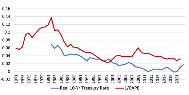
Source: dividend yield: http://www.econ.yale.edu/~shiller/data.htm; Federal Reserve Bank of Cleveland, 10-year real interest rate, retrieved from FRED, Federal Reserve Bank of St. Louis; https://fred.stlouisfed.org/series/REAINTRATREARAT10Y, April 29, 2023.

Figure 1. The safe real interest rate and earnings-price ratio.

then followed by some acceleration until the mid-2000s. The productivity numbers therefore are also consistent with some of the capital gains during this period as being due to changes in the required return on stocks.

The rise in the earnings price ratio starting in 2000 is much more difficult to interpret because of the severity of the two most recent recessions. While the real interest rate continued to fall, it is much more difficult to infer what was happening to risk premia and productivity growth (e.g. see Gordon & Hassan, 2022 and Fernald et al., 2023 ).

3. General Equilibrium Model

Consider the problem of a life-cycle consumer who will work for N periods and consume for T-N more periods while retired. The consumer’s problem can be written as

$\max V_{jt}={\displaystyle \underset{i=j}{\overset{T}{\sum }}\left({\beta }^{i-j-1}\frac{C_i^{1-\rho }}{1-\rho }\right);}\text{s}\text{.t}\text{.}{\displaystyle \underset{i=j}{\overset{N}{\sum }}\frac{Y_i}{R_{i-j+t}^{i-j-1}}}={\displaystyle \underset{j=1}{\overset{T}{\sum }}\frac{C_i}{R_{i-j+t}^{i-1}}}$ , (1)

where β is the discount factor, ρ is the degree of relative risk aversion, C_j and Y_j are planned consumption and income at different ages, and R_t is one plus the interest rate. The only stores of value in this economy are shares in a “tree,” s, where the price of the tree at time t is P_t, and consumers can buy partial shares in the tree. The return on a share of the tree at time t is (MPK_t + P_t+1)/P_t, which is equal to R_t. This section, looks only at stationary equilibria, where the interest factor, R, is constant over time. The model does allow for growth in total factor productivity at the rate g, so that the price of the tree at a stationary equilibrium is given by the dividend discount formula,

$P_t=\frac{MP{K}_{t}G}{R_t-G},\text{where}G=\left(1+g\right)\text{and}{R}_t=\frac{MP{K}_{t}G}{P_t}+G$ (2)

Constant relative risk aversion is a special case of Epstein-Zinn preferences, where consumption at any age, j, is given by (see for example Zhang, Hardy, & Saunders, 2018 and the appendix for derivations):

$\begin{array}{l}{C}_j^{*}=\frac{W_j}{D{F}_j}\text{,where}{W}_j=s_j{P}_t+{\displaystyle \underset{i=j}{\overset{N-j}{\sum }}\frac{Y_i}{R^{i-j}}}\text{for}j\le N\text{and}{s}_j{P}_t\text{for}j>N\text{where}\\ D{F}_j={\displaystyle \underset{i=j}{\overset{T+j-1}{\sum }}{\left({\beta }^{i-j}{R}^{i-j}\right)}^{\frac{1}{\rho }}/R^{i-j}},\text{sothat}\end{array}$ (3)

$C_{j+1}^{*}={\left(\beta R\right)}^{\frac{1}{\rho }}{C}_j^{*}\text{and}{V}_j^{*}=\frac{W_j^{1-\rho }D{F}_j^{\rho }}{1-\rho }.$ (4)

The term DF_j can be thought of as a kind of discount rate, that reflects time preference and intertemporal substitutability. For example, if βR = 1, the 1/DF term is the present discounted value of a $1 for T − t periods, and consumption is a constant over time. If βR > 1 (pure time preference is less than the interest rate), then the discount factors is greater than the PDV of a constant income stream, reducing current consumption relative to future consumption. The larger the elasticity of intertemporal substitution, the greater the bias toward the present in this case.

A general equilibrium in the model is given by a price of the tree such that the total number of shares held is equal to 1, and consumers’ choices of consumption over all ages sum to income. There is no population growth and one representative consumer at each age. Total wage income is equal to the size of the population, N, so that the average wage is equal to 1. The assumed pattern of life-cycle income is roughly similar to those in Guvenen et al. (2022) or Feiveson and Sabelhaus (2019) , where income first doubles with age and then declines by 2 percent per year for the last 10 years of work.

The remaining parameters of the model are chosen to be close to those in R&S: 1) For the “early” period: working life of 48 years with 11 years in retirement and total factor productivity growth of 1.51 percent. In the later period: working life of 46 years with 19 years in retirement and total productivity growth of 0.7 percent. The return to the tree, MPK, is 23, so that labor’s share is between 67 and 68 percent. Pure time preference is assumed to be 2 percent. This analysis is less interested in the effects of uncertainty, so as opposed to Rachel and Summers (2019) , there is no uncertainty, including survival uncertainty. The parameters and equilibrium interest rates are given in Table 1.¹

The equilibrium interest rate looks high relative to that in Rachel and Summers (2019) . Their base line 1970 model has a real interest rate of 4.5 percent. Some of this difference is due to the assumption of a varying age-income profile for workers. For example, if the two models are solved assuming homogeneous workers so that the wage is one over the working life (as in R&S), the equilibrium interest rates fall to 1.080 and 1.051 for the two time periods, respectively.

The point of the model, however, is to illustrate how real factors can cause a decline in the market discount rate that is roughly in line with that in R&S. Table 2

Table 1. General equilibrium model: parameters and equilibria.

Table 2. Private sector effects on R*: 1970-2017.

compares the two models in terms of the effects of increasing retirement age and slowing productivity on the interest rate. The two models appear to capture similar effects for the increase in the length of retirement and the slowdown in total factor productivity growth.

4. Welfare Effects of Unexpected Capital Gains

The analysis now turns to how unexpected capital gains affect individual workers, whether such gains qualify as an increase in Hicksian income. It should be noted at the outset that in a perfect foresight world none of the capital gains analyzed in the general equilibrium model would affect workers’ welfare. But given the vast literature on excess volatility (for a recent example, see Wehrli & Sornette, 2022 ) and the facts that papers such as R&S are trying ex post to explain the secular decline in interest rates, it seems plausible that some of the non-recurring capital gains over the last 50 years have been unexpected. This section analyzes how the welfare of the life-cycle workers in the general equilibrium model are affected by such unexpected capital gains.

The analysis starts by determining the effects of an unexpected decrease in the interest rate on the future value of $1 worth of shares of the tree in k years, FV^k+1. Let R_t reflect the increase in the future value of shares following an unexpected increase in P_t+1, that permanently lowers R_t+j, j > 0.

$\begin{array}{l}F{V}^{k+1}=R_t{R}_{t+1}^k,\text{where}\\ R_t=\frac{P_{t+1}+MP{K}_{t+1}}{P_t},\\ \text{note}G{P}_{t+j}=P_{t+j+1}\text{and}GMP{K}_{t+j}=MP{K}_{t+j+1}\text{,sothat}\\ \text{and}{R}_{t+1}=\frac{G\left(P_{t+1}+MP{K}_{t+1}\right)}{P_{t+1}}=G+\frac{MP{K}_{t+1}}{P_{t+1}}\end{array}$ (5)

$\begin{array}{l}\frac{\text{d}F{V}^{k+1}}{\text{d}{P}_{t+1}}=\frac{R_{t+1}^k}{P_t}-\frac{k{R}_t{R}_{t+1}^{k-1}MP{K}_{t+1}}{P_{t+1}^2};\text{forsmallchangesin}{P}_t,R_t=R_{t+1}\\ \frac{\text{d}F{V}^{k+1}}{\text{d}{P}_t}=\frac{R_{t+1}^k}{P_t}\left(1-\frac{kMP{K}_{t+1}}{P_{t+1}}\right)=\frac{R_{t+1}^k}{P_t}\left(1-k\left(\frac{R_{t+1}-G}{G}\right)\right)\end{array}$ (6)

Let k^* be the value of k such that the future value of the $1 worth of shares k + 1 years from now is unaffected by unexpected increase in P_t, or where the unexpected capital gain is just offset by the lower return on shares over the next k years. From (6)

$k^{*}=\frac{G}{R_{t+1}-G}\text{.}$ (7)

From (6), for a given R, k^* rises with G¸ and for a given G, k^* falls with R. It also suggests that the more of the return from shares that is due to recurrent capital gains, the greater k^*. This makes intuitive sense because when R_t-G is low, more of the present value of a share is based upon future dividends, which are more sensitive to changes in the discount rate than are closer dividends.

The information in Table 1 implies k^* for the 1970 and 2017 general equilibria are 12.6 and 18.7 years, respectively. The increase in k^* between 2017 and 1970 is due to both a drop in R_t+1 and in R_t+1-G In a discrete-time model, this implies that $\frac{\text{d}F{V}^{k+1}}{\text{d}{P}_t}\frac{>}{<}0$ , as $k\frac{<}{>}trunc\left(k^{*}\right)$ . So, these numbers imply that an unexpected capital gain would raise the future purchasing power over any good during the next 12 years, for the 1970 equilibrium and the next 18 years for the 2017 equilibrium. Thus, unexpected capital gains have substantial effects on future purchasing power.

But this result is not sufficient for determining the welfare effect on workers. In the model, workers are accumulating shares up until retirement, so that any increase in the future value of current assets for workers is at least partially offset by the higher price on new shares purchased and concomitantly lower interest rate on these new shares. One can see this by looking at the effect of an unexpected, but permanent reduction in the market discount rate on indirect utility. From (3)

$\begin{array}{l}{V}_j^{*}=\frac{W_j^{1-\rho }D{F}_j^{\rho }}{1-\rho }\\ \frac{\text{d}{V}_j^{*}}{\text{d}R}={\left(\frac{D{F}_j}{W_j}\right)}^{\rho }\frac{\text{d}{W}_j}{\text{d}R}+\frac{\rho V_j^{*}}{D{F}_j}\frac{\text{d}D{F}_j}{\text{d}R}\text{.}\end{array}$ (8)

The first term is unambiguously negative, while the second is positive (shown in the appendix). The first term captures the effects of the unexpected capital gain on wealth and the second the effect of the change in the rate of return for a given wealth. Retirees are always selling assets, so the net effect of an unexpected rise in the price of shares must be positive, and conversely, young workers with no financial wealth must be worse off with a permanent increase in the price of shares. More generally, there is no neat solution for resolving the ambiguity in the change in welfare for workers with some financial wealth.

But, a numerical simulation of the model can, and to the extent that it captures the life-cycle dynamics of industrialized countries it can shed light on the likely welfare effects of unexpected capital gains on different cohorts of workers. Specifically, starting from the 2017 general equilibrium, all workers with more than 7 years until retirement are made worse off by a reduction in R. This result is sensitive to the assumption of the age-income profile. If it is assumed, as it is R&S, that workers of all ages are equally productive, the equilibrium interest rate falls from 6.1 percent to 5.1 percent, and k^* rises from 18.7 to 22.7. Consequently, an unexpected capital gain benefits more workers, in particular any worker with more than 11 years until retirement. In either case the substantial majority of workers are made worse off.

5. Conclusion

The analysis in this paper is in many ways similar to capturing the welfare effects of a change in relative prices through the use of a price index. When the price of future goods rises because of an unexpected fall in the interest rate, workers in general are worse off because their income streams are shorter than their planned consumption streams. Some of this loss, however, if offset by the non-recurring capital gains on their holding of financial assets, these capital gains increase the workers’ purchasing power over future goods. The analysis has shown that there is a complicated tradeoff between the gains on financial assets versus the loss in the purchasing power of the future income over planned future consumption. The numerical simulation showed that the vast majority of workers, however, are worse off.

The policy implications of the analysis suggest that for most workers many unrealized capital gains do not represent Hicksian income nor an increased “ability to pay” taxes. But even life-cycle workers sometimes have to realize capital gains: e.g. for emergency needs, for lumpy consumption, to rebalance portfolios. The taxation of these kinds of gain seems inequitable, since in many cases the gains reflect a loss in Hicksian income. Designing a tax law that alleviated this inequity would be difficult, particularly because not all capital gains are due to unexpected reductions in the real interest rate. But one could imagine treating capital gains in a way similar to the treatment of early withdrawals from IRAs: reducing the tax rate on realized gains that are used to pay medical expenses, college tuition, home purchases and “rollovers” as part of portfolio rebalancing.

Appendix of Derivations

1) Earnings-Price Ratio

The market value of a firm can be written as: $PS=ES/r_S+NPVGO$ , where P is the stock price, S is the number of shares, E is the firm’s earnings per share, r_S is a risk-adjusted interest rate on the stock and NPVGO is the net present value of growth opportunities.

$\frac{P}{E}=1/r_S+\frac{NPVGO}{ES}.$

Thus, the larger the numerator of the last term relative to the denominator the more the P/E ratio will exceed 1/r_S and the less E/P ratio will be below r_S

2) Indirect Utility Function

$V_j={\displaystyle \underset{i=j}{\overset{T+j-1}{\sum }}\left({\beta }^{i-j}\frac{C_i^{1-\rho }}{1-\rho }\right)}$ . From Zhang, Hardy and Saunders (2018: p. 5)

$\begin{array}{l}{C}_j^{*}=\frac{W_j}{D{F}_j}\text{,where}D{F}_j={\displaystyle \underset{i=j}{\overset{T+j-1}{\sum }}{\left({\beta }^{i-j}{R}^{i-j}\right)}^{\frac{1}{\rho }}/R^{i-j}}\\ ={\displaystyle \underset{i=j}{\overset{T+j-1}{\sum }}{\beta }^{\frac{i-j}{\rho }}{R}^{\frac{\left(i-j\right)\left(1-\rho \right)}{\rho }}}\end{array}$

$\begin{array}{l}{C}_{j+1}^{*}={\left(\beta R\right)}^{\frac{1}{\rho }}{C}_j^{*},\text{so}\\ V_j^{*}=\frac{{\displaystyle \underset{i=j}{\overset{T+j-1}{\sum }}\left({\beta }^{i-j}{\left({\left(\beta R\right)}^{\frac{i-j}{\rho }}\frac{W_j}{D{F}_j}\right)}^{1-\rho }\right)}}{1-\rho }\end{array}$

Consider the last term in the summation, which can be written as:

${\beta }^{T-1}{\left({\left(\beta R\right)}^{\frac{T-1}{\rho }}\frac{W_j}{D{F}_j}\right)}^{1-\rho }={\beta }^{T-1}{\left(\beta R\right)}^{\frac{\left(T-1\right)\left(1-\rho \right)}{\rho }}{\left(\frac{W_j}{D{F}_j}\right)}^{1-\rho }={\beta }^{\frac{T-1}{\rho }}{R}^{\frac{\left(T-1\right)\left(1-\rho \right)}{\rho }}{\left(\frac{W_j}{D{F}_j}\right)}^{1-\rho }$

${\beta }^{\frac{T-1}{\rho }}{R}^{\frac{\left(T-1\right)\left(1-\rho \right)}{\rho }}$ is the same as the last term in $D{F}_j$ and similar for all the other terms, so

$V_j^{*}=\frac{D{F}_j{\left(\frac{W_j}{D{F}_j}\right)}^{1-\rho }}{1-\rho }=\frac{W_j^{1-\rho }D{F}_j^{\rho }}{1-\rho }$

3) Unexpected Capital Gain and Welfare

$\begin{array}{l}D{F}_j={\displaystyle \underset{i=j}{\overset{T-j}{\sum }}{\left({\beta }^i{R}^i\right)}^{\frac{1}{\rho }}/R^i}\text{,}\text{or}\\ ={\displaystyle \underset{i=1}{\overset{T-j}{\sum }}{\beta }^{\frac{i}{\rho }}{R}^{\frac{i\left(1-\rho \right)}{\rho }}}\text{,}\frac{\text{d}D{F}_j}{\text{d}R}\frac{<}{>}0,\text{as}\rho \frac{>}{<}1,\text{sothat}\\ \frac{\rho V_j^{*}}{D{F}_j}\frac{\text{d}D{F}_j}{\text{d}R}>0\end{array}$

NOTES

¹Details of all calculations and results in Tables 1&2 are in the Excel sheet, available at: https://docs.google.com/spreadsheets/d/1Ec-xYBUF2oEAlu6UUp3Ckovv9jytlq3C/edit?usp=sharing&ouid=108104673539474975338&rtpof=true&sd=true.

Conflicts of Interest

The author declares no conflicts of interest regarding the publication of this paper.

References

[1]	Feiveson, L., & Sabelhaus, J. (2019). Lifecycle Patterns of Saving and Wealth Accumulation. Finance and Economics Discussion Series, #10, Divisions of Research & Statistics and Monetary Affairs Federal Reserve Board. https://doi.org/10.17016/FEDS.2019.010
[2]	Fernald, J., Inklar, R., & Ruzic, D. (2023). The Productivity Slowdown in Advanced Economies: Common Shocks or Common Trends. Federal Reserve Bank of San Francisco Working Paper 2023-07. https://doi.org/10.24148/wp2023-07
[3]	Gordon, R., & Sayed, H. (2022). A New Interpretation of Productivity Growth Dynamics in the Pre-Pandemic and Pandemic Ear of the US Economy, 1950-2022. NBER Working Paper 30267. https://doi.org/10.3386/w30267
[4]	Guvenen, F., Kaplan, G., Song, J., & Weidner, J. (2022). Lifetime Earnings in the United States over Six Decades. American Economic Journal: Applied Economics, 14, 446-479. https://doi.org/10.1257/app.20190489
[5]	Hicks, J. R. (1964). Value and Capital (2d ed.). Oxford University Press.
[6]	Nichols, D. (1971). A New Measure of Income from Wealth. Cowles Foundation Disc. Paper No. 321.
[7]	Nichols, D. (1974). The Investment Income Formula of the American Economic Association. The American Economic Review, 64, 420-426.
[8]	Rachel, L., & Summers, L. (2019). On Secular Stagnation in the Industrialized World (pp. 1-54). Brookings Papers on Economic Activity. https://doi.org/10.3386/w26198
[9]	Simons, H. C. (1938). Personal Income Taxation. University of Chicago Press.
[10]	Tobin, J. (1974). What Is Permanent Endowment Income? The American Economic Review, 64, 427-432.
[11]	Wehrli, A., & Sornette, D. (2022). The Excess Volatility Puzzle Explained by Financial Noise Amplification from Endogenous Feedback. Scientific Reports, 12, Article No. 18895. https://doi.org/10.1038/s41598-022-20879-0
[12]	Zhang, S., Hardy, M., & Saunders, D. (2018). Epstein-Zin Preferences in Life-Cycle Applications: Uncertain Lifetime and Consumption Smoothing. https://doi.org/10.2139/ssrn.3245960