The Volatility of Capital Structure in Brazil—An Empirical Analysis ()
1. Introduction
Gama Boaventura, Rodrigues Cardoso, Simoni da Silva, & Santos da Silva (2009) apud Friedman (1962), in the famous work capitalism and freedom, argue that the company has a single objective: economic performance. Smith (2003), cited by Gama Boaventura, Rodrigues Cardoso, Simoni da Silva, & Santos da Silva (2009) , clarifies that, according to shareholders’ theory, they advance capital, so that managers use it only in what they authorized, while in the stakeholder theory, managers have obligations to shareholders and stakeholders. Thus, the problems of profit maximization arise, which develop trade-off, pecking order, all these and others, trying to explain this maximization.
The study of capital structures has always been the subject of great debate and (Sarkar, 2017: p. 64) confirms it by mentioning that “the capital structure and its influence on the financial performance and overall value of the company have been a matter of considerable attention among finance scholars since the pivotal work of (Modigliani & Miller, 1958) ”.
Former Brazilian President Fernando Henrique Cardoso (1995-2002), in a speech at a conference in Washington on April 21, 1995, called this influence the “most political of economic issues” (Cardoso, 1995) .
The Brazilian market was chosen between 2003 and 2016, preferably for its entire political context, and for the great influence on the financial market, according to (Alves Teixeira & Costa Pinto, 2012: p. 923) when they state that “Brazil went through the cycle of longest growth in the last three decades.” The volatility of capital structures as a study of the static trade-off was questioned by DeAngelo & Roll (2015: p. 373) , as follows: “The view that corporate leverage is stable permeates the empirical literature on capital structure and fosters the belief that the main puzzle that researchers face is explaining the variation between companies in leverage.”
The purpose of this article is to analyze whether “the instability of the corporate capital structure over time is a rule (static trade-off)” and whether “stability or instability generates profitability for Brazilian companies”.
This research innovates by studying the volatility of the way companies finance themselves and not in intensity or just in determinants.
It was also innovative when questioning the trade-off theory regarding its stability in an emerging market like Brazil, as the vision of stability already permeates the entire literature since 1980.
2. Literature Review
In order to compose a theoretical framework capable of supporting this study, some theories and approaches related to the subject are presented. This set of ideas that make up the theoretical contribution of this study are explained and discussed below.
Capital structure refers to the way a company seeks to determine financial resources to finance its activities. In this case, shares, shareholders’ capital, debts, are some of the options on how to finance.
Therefore, this study was developed from the theories of (Modigliani & Miller, 1958) . After Modigliani and Miller, discussions on capital structures were the Trade-off Theory (DeAngelo & Masulis, 1980) and (Bradley et al., 1984) , Pecking order Theory (Myers, 1984) , (Graham & Harvey, 2001) agency costs (Jensen & Meckling, 1976) .
Initially, there is the traditional Theory that began with Durand (1952) , from studies on asset financing and the costs incurred in this financing. In the Modigliani & Miller Approach, the suggestion is that for owners, the cost of capital is just the interest rate on bonds. Thus, some assumptions are stipulated for the formulation of their proposals, as (Jarosa & Bartosova, Viera, 2015; Esperança & Matias; 2010; Carvalho 2016) , being perfect capital market; financing only for bonds and shares; obtaining credit is the same for all companies; non-existent bankruptcy risk; the costs of financial difficulties are nil, among others.
Then, there is a set of theories that support the theme, such as the Tax Effect Theory, which, according to Modigliani & Miller (1963) , answers several questions in their 1958 article, when market imperfections were recognized, including the effects of taxes on income of companies. Furthermore, they considered that companies should not always use as much debt as possible in their structures at all times. They also suggested other types of debts, taking into account the personal income tax.
Trade-offs emerged as a consequence of the tax effect of Modigliani & Miller (1963) , being cited by authors such as Warner (1977) , Miller (1977) , DeAngelo & Masulis (1980) , Myers (1984) . However, his greatest work is attributed to Bradley et al. (1984) , considered the author of the standard trade-off model, in the view of Frank & Goyal (2008) . Still, the Trade-off (Fama & French, 2002) applies effectively when companies are looking for optimal leverage, weighing the costs and benefits of adding a dollar to debt in this case. The benefits are tax deductibility of interest and reduced free cash flow problems. The costs are the possibility of bankruptcy and possible agency conflicts.
It is worth noting that the Trade-off is defended because it is static, according to Amaral, Paulo (2011) apud Altman (1984), as they balance due to financial stress. Furthermore, as the trade-off does not contain a goal adjustment, according to Frank & Goyal (2008) , the literature has divided the trade-off into static and dynamic. This trade-off volatility, Dudley (2007) states that it is more advantageous due to the readjustment of debt ratios.
The Information Asymmetry Theory, also known as Signaling Theory, was developed by Ross (1977) , Akerlof (1970) and Leland & Pyle (1977) , having as main characteristic the information, usually incomplete, that the financial market already has. Thus, companies that standardize information generally have a lower market value (Myers, 2001) and to increase the value of these companies, Rajan & Zingales (1995) advocate the inclusion of large shareholders in the board of directors. Glenn Hubbard (1990) cites it as just a market failure, not a theory itself.
The Pecking order Theory was initiated by Donaldson in 1961 which was possibly the precursor of a financing hierarchy, but Myers (1984) was one of the great early works on this order. To Frank & Goyal (2009) , Fama & French (2002) and Harris & Ravis (1991) , the pecking order theory is based on the asymmetric information theory. In pecking order, companies pay higher dividends and more profitable companies have fewer loans, due to greater internal resources. Companies with more investments have lower dividend payments and those with few tangible assets tend to have more debt, according to Fama & French (2002) , Myers (2001) and Harris & Ravis (1991) .
Agency Theory is a model initially proposed by Jensen & Meckling (1976) with three pillars: property rights, agency conflicts between owners and managers and finances. For Frank & Goyal (2008) , this conflict arises when for a new external financing manager has to explain the details of the companies’ projects to external investors, exposing the monitoring of these investors. It is from this theory that the Theory of Capital Agency arises, in which managers tend to continue with the operations of companies, even if shareholders prefer debt (Harris & Raviv, 1991; Strebulaev, 2007) and also puts as a consequence the bankruptcy cost in this conflict.
And there is also the Debt Agency Theory, which deals with the conflict between creditors and shareholders, when these are not resolved solely on the basis of the contract (Harris & Raviv, 1991) . Furthermore, the conflict between shareholders and creditors only arises when there is a “standard risk”, that is, if there is a risk of breach of contract (Myers, 2001) .
The Market Timing Theory is more recent and came to try to explain the shortcomings of the previous ones. It is known due to the study by Baker & Wurgler (2002) , being just a complement to other theories according to Frank & Goyal (2009) . Graham & Harvey (2001) state that market timing is when managers make an “adjustment to the market”.
As for the Takeover Theory, its classification is based on theories of dispute of control, in which the value of the company is related to the ability of a company manager to manipulate the method and the probability of success of an acquisition attempt, changing the fraction of the assets he owns according to Harris and Ravis in 1988 and Stulz in 1988.
The Volatility of Capital Structures, scope of this article, arises in the discussion of Trade-off dynamics. According to Myers (1984) , when companies reach the desired target, they tend to stabilize, not changing much in the long term. However, Minton & Wruck (2001) found that low leverage is largely a transient phenomenon. In studies by Lemmon, Roberts, & Zender (2008) and Frank & Goyal (2008) , the conclusion is that companies remain with the same leverage for long periods. But other authors cited by Myers (1984) such as Marsh in 1982 and Taggart in 1977 showed that British companies adjust to a leverage target.
In this regard, DeAngelo & Roll (2015) carried out research in the USA, between the years 1950 and 2008, on companies listed on the Dow Jones Industrial Average, which answered several questions arising from the consistency or not of companies deviating from their goals under different forms of segmentation and concluded that “episodes of leverage stability in individual companies occasionally arise. This stability occurs mainly with low leverage and is practically always temporary”, that is, the “Static Trade-Off” theory is an exception. Chong & Kim (2019) analyzed volatility between 2006 and 2016 in South Korea and concluded that the Korean companies’ capital structure is not stable over time and that companies with higher capital structure volatility are characterized by a higher level of financial vulnerability.
In Europe, Campbell & Rogers (2018) researched volatility in the United Kingdom, Germany, France and PIIGS (Portugal, Italy, Ireland, Greece and Spain), concluding that companies with more volatile debt tend to be smaller and less profitable, while companies with a stable capital structure generally have low cash volatility from operating and investing activities.
In Brazil, there is a study by Tristão & Sonza (2019) , in which companies listed on the BolsaBalcãoBrasil (B3) from 1995 to 2015 were analyzed. The conclusion reached is that there is also instability in leverage.
3. Methodology
3.1. Research Hypotheses
Based on the literature review, the research hypotheses (1 - 17) were formulated, together with the description of the variables, which seek to respond to the impact of the volatility of capital structures (1 to 6) and the impact on accounting leverage (7 to 17).
1) There is a negative relationship between return on assets (ROA) and volatility.
2) There is a negative relationship between the size and volatility of capital structures.
3) There is a positive relationship between small companies and the volatility of capital structures.
4) There is a positive relationship between change of assets and the volatility of capital structures.
5) There is a negative relationship between market-to-book growth opportunities and the volatility of capital structures.
6) There is a positive relationship between sales growth and volatility.
7) There is a positive relationship between return on equity (ROE) and accounting leverage.
8) There is a negative relationship between return on assets (ROA) and accounting leverage.
9) There is a negative relationship between dividends paid and accounting leverage.
10) There is a positive relationship between size and accounting leverage.
11) There is a positive relationship between size measured by net worth and accounting leverage.
12) There is a negative relationship between small businesses and accounting leverage.
13) There is a positive relationship between asset tangibility and accounting leverage.
14) There is a negative relationship between sales growth and accounting leverage.
15) There is a negative relationship between market-to-book growth opportunities and accounting leverage.
16) There is a negative relationship between change assets and accounting leverage.
17) There is a negative relationship between capex and accounting leverage.
The research hypotheses will be answered in subitem 4.1 in Table 7 and Table 8 of this article.
3.2. Database
The article used data from the Economática software, with information from the stock exchange (B3). The data collected refer to the period from 2003 to 2016, chosen based on an apparent financial and exchange rate stability. Data from the companies’ financial, accounting and market statements were used.
The data are consolidated, in dollars, without inflation updating, collected on December 31st, or on the last available day in December, being in some cases, December 30th or 29th, however, they are validated under Brazilian legislation.
Market values, is the share price, were chosen on the last available day, most of which are December 31st. Version 13 of Stata software and Microsoft Excel were used for statistical and graphic analysis.
The initial database contained 7423 observations. All financial companies, banks and the like were removed accordingly (Lucey & Zhang, 2011: p. 3) . Companies whose balance sheets were negative or with zero value were also excluded, so that there was no negative leverage or no leverage. Companies that did not have a quotation in the year of analysis, or that did not have information on the number of shares traded on the market, were also removed. The final base contains 572 companies, 5087 observations, from the most varied sectors of activity.
3.3. Dependent Variables
1) The. Volatility of capital structures—This was followed by the DeAngelo & Roll (2015) research, as a dependent variable for the analysis of capital structures. Other authors have already used a similar variable, such as Lamont et al. (2001) , when using the standard deviation of the financial constraint factor, which was used as a basis for the analysis of capital structures and stock returns in Korea by Chong & Kim (2019) .
2) Accounting leverage—Or simply debt, has been studied since the famous works of (Modigliani & Miller, 1963; DeAngelo & Masulis, 1980; Myers, 1984; Jensen & Meckling, 1976) .
Accounting leverage was chosen and not market leverage, as well as Frank & Goyal (2009) due to the fluctuation of the financial market. To analyze the trade-off theory and its stability (or not), the total leverage and its volatility were used, and not its intensity.
3.4. Independent Variables
Frank & Goyal (2009) states that there are “essential factors”, that is, determinants that in their research represented 27% of the leverage variation, these being “macro determinants”: Activity Sector; Nature of Assets; Return or Profits; Company size; Growth and Inflation. It should be noted that in this article inflation was not analyzed.
In the analysis of return or profit, the variables were:
1) The. Return on Equity (ROE)—Represents the return of the partners for each monetary unit invested in the company’s equity, according to Ferrari and Luiz (2014) . Although ROE is not a fully efficient measure to measure corporate performance, studies similar to this variable were followed, such as Lara & Mesquita (2008) and Kumar & Sharma, 2011 .
2) Return on Assets (ROA)—Variable generally used to measure short-term risks Frank & Goyal (2009) ; this variable is also used to measure the profitability of companies, according to Booth et al. (2001) and Lemmon, Roberts, & Zender (2008) .
3) Dividends (DIV)— Frank & Goyal (2009) state that companies that pay dividends have less leverage than companies that do not. Other studies have included it, such as Fama & French (2002) and Lemmon, Roberts, & Zender (2008) .
To analyze the size of the company, the analysis considered three (3) variables:
4) Logarithm of Assets (Log_Tam)—Used as a variable to calculate the size of companies, as in Lemmon, Roberts, & Zender (2008) . Titman & Wessels (1988) state that large companies should be more leveraged and have lower costs to issue new equity. The authors also state that large companies use their assets as collateral to pay debts. Regarding the volatility of capital structures, Campbell & Rogers (2018) conclude that large companies tend not to significantly change their debts.
5) Logarithm of PL (Log_PL)—As well as a measure of size, this variable was used as Perobelli & Fama (2003) and Sonza & Kloeckner (2014) . The objective is to identify not only large companies measured by assets, but also large companies measured by the size of their net worth, as it is possible to capture companies that have little debt, but have a large net worth.
6) Small Sized Dummy (SZ)—As a control and in contrast to Leary’s (2009) maturity variable, this variable was used according to Campbell & Rogers (2018) , who analyzed it to capture the difficulties that smaller companies may have in accessing debt.
To measure the nature of the assets, the following determinants were verified:
7) Tangibility of assets (Tang)—It is the company’s ability to use collateral debt, that is, use guarantees to honor debts according to Kieschnick & Moussawi (2018) , Palacín-Sánchez, Ramírez-Herrera and Pietro (2013) .
8) Sales Growth (SaG)—It is a revenue growth variable. It was included in this, according to Valle (2008) , to analyze the risk of underinvestment due to agency problems; other studies have also related it as Brito et al. (2007) .
As for growth, it was analyzed with the following variables:
9) Market-to-book (MtK)— Kieschnick & Moussawi (2018) used this variable as a proxy to capture a company’s growth prospects. Other studies used this variable, such as Rajan & Zingales (1995) and Lemmon, Roberts, & Zender (2008) .
10) Change Assets (ChA)— Frank & Goyal (2009) classify changes in assets as one of the variables in the group of growth variables; they reduce cash problems, increase agency problems because certain companies value shareholders’ investments more. Campbell & Rogers (2018) , when analyzing the volatility of capital structures, observed that companies with more volatile debt also alternate their assets.
11) Capital Expenditure (Capex)—Still in the growth analysis, it was used according to Frank and Goyal (2009) and Darwin & Aquino (2009) , the latter being in emerging economies, in the case of the Philippines. They concluded that companies depend more on equity than debt to finance their capital expenditures.
Finally, we sought to analyze volatility and leverage in terms of the activity sector, which Frank & Goyal (2009) classifies as an industrial sector.
12) Activity Sector—Dummy variables are generally used to control, increase the significance of other variables, etc. Dummy variables were chosen for the sector of activity, as in Titman & Wessels (1988) . Campbell & Rogers (2018) also included industry dummy variables to relate to the volatility of capital structures and operating leverage. This article classified them as industry, service, commerce, as described by (B3) BolsaBalcãoBrasil (Table 1).
3.5. Statical Model
Panel data was chosen due to the characteristic of the research being over a long period and due to the heterogeneity, informative diversity, variability, less collinearity and more adequate to examine changes according to Baltagi (2005) .
In choosing the models, Pooled OLS (OLS), fixed effects (FE) and random effects (RE) were used as static models and the Generalized Methods of Moments – GMM for the dynamic model.
The least squares method or OLS and GMM presupposes some assumptions for the model to be valid. Thus, the validity of the model was verified, according to Gujarati & Porter (2011) , regarding multicollinearity, autocorrelation and homoscedasticity.
After all of the proposition tests, the model used was the GMM due to the amount of statistically significant variables and, below, the results for the GMM model were listed.
Table 2 of this article, described below, presents the commerce, services and industry companies, classified as a dummy variable described in line L of item 3.4 and is in accordance with studies by Campbell & Rogers (2018) , among other studies. The database was scaled by total assets, with Largest Reduction being the companies that reduced their capital structures by 15% or more, which reduced from 5% to 15% in the group B, those that reduced or increased by up to 5% in group C, those that increased from 5% to 15% in group D, those that increased by more than 15% in Largest Increase.
![]()
Table 1. Calculation of the independent variables used in the two models.
Source: Author’s own.
![]()
Table 2. Changes in capital structure.
Source: Author’s own.
For multicollinearity, the VIF test was performed according to Table 3, which shows when an estimator is biased in terms of its variance. The closer it is to 1, the lower the chance of having multicollinearity, from the perspective of Gujarati & Porter (2011) .
Source: Author’s own.
According to Table 3, the models with the accounting leverage variable in the scalar size variable “largest reduction”, “B”, “D” and “Largest Increase”, the independent variable Log_PL was removed due to multicollinearity.
The linear association of the variables was analyzed in Table 4 and Table 5 through Pearson’s correlation according to Figueiredo Filho et al. (2014) .
For the autocorrelation test in the dynamic GMM model, Arellano-Bond (1990) proposed a test of 1st and 2nd residual differences for validation, in which the errors would not be correlated in series. Fonseca, Santos, Pereira, Camargos, (2018) apud Bueno (2008) explain that the first lag eliminates the fixed effect of endogenous variables and the second consists of using it as an instrument, followed by the use exogenous as instruments of themselves.
To validate the GMM model, the Sargan test for endogeneity was performed, according to Arellano (2002) .
4. Results
The database presented 5087 observations, which for descriptive analysis was not divided into the scalar variable size.
The average leverage is 55%, with a minimum of 0% and a maximum of 100%, with a standard deviation of 23% from the average, that is, the average debt of the sampled companies is around 42% to 123%, very similar to Portugal and Greece, according to the study by (Campbell & Rogers, 2018) with an approximate average of 40%.
![]()
Table 4. Pearson’s correlation, volatility of capital structures.
Source: Author’s own.
![]()
Table 5. Pearson’s correlation, accounting leverage.
Source: Author’s own.
Analyzing Table 6, companies listed on B3, in the analyzed period (2003-2016) increased their assets by 7.32% compared to the previous year (0.03 log), higher than the average growth of Brazilian GDP, which was 2.5% according to IBGE data, Brazilian Institute of Geography and Statistics. This apparent growth is not consistent with the non-distribution of dividends (dividends paid on net income), which in principle can only be a policy of non-distribution of dividends, or it can also reveal that they only got into debt.
The sample is divided into three large groups: industry 33%, commerce 18% and service 47%, following the IBGE division, except for the agriculture/livestock division, which was not significant for the analysis carried out. The average size of company assets is ?,150,000,000.00 (two thousand one hundred and fifty billion euros) or (two thousand five hundred billion dollars).
Graphic 1 presents the predictive power of a given cross-section for the sequence of future cross-sections according to DeAngelo & Rool (2015) .
Source: Author’s own.
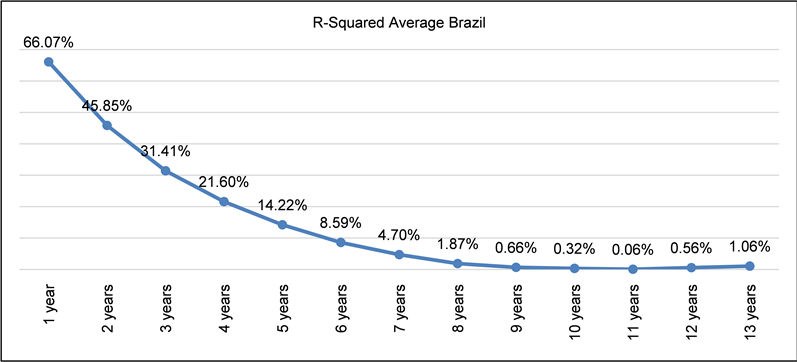
Graphic 1. Representativeness of the volatility of capital structures in Brazil. Source: Author’s own.
To calculate the average R2, or average R-Squared for the different cross-sections, the first step was to calculate the annual leverage of all companies in the database. Then, the correlation between leverage in pairs of years of the sample was obtained, such as one year, 2003/2004, 2004/2005, 2005/2006. Subsequently, the difference in years was increased, 2003/2005, 2003/2006, two years, until reaching the 13-year difference, 2003/2016. Finally, the average of the R-Squared pairs of years of the sample correlations is calculated. The closer to 1, the more volatile the capital structures are.
Campbell & Rogers (2018) analyzed the volatility in Europe between the years 2006 to 2016, which is different from the database used in this article (2003-2016), so when comparing the results between Brazil and Europe, we conclude-The predictive power of a given cross-section for the sequence of future cross-sections after 10 years was approximately 20% in Europe, while in the Brazilian market it was close to 0%, as the Brazilian market is highly volatile, as the initial study by (DeAngelo & Roll, 2015) , on the non-stability of Trade-Off.
In Graphic 2, leverage was analyzed individually for the largest companies in the three sectors of the analysis, as shown in Graphic 2, being Eletrobras - CentraisElétricasBrasileiras S.A., Petrobras - PetróleoBrasileiro S.A. for the industry sector, Pão de Açúcar and Fibria for the commerce sector, and Telemar for the service sector, the latter is specific to the telecommunications sector.
It is seen in all the companies mentioned, the great volatility of the indebtedness, which proves that the theory of Trade-Off was not applied to these companies, confirming the R-Squared forecast graph.
In the joint analysis between the individual graphs of the companies and the volatility, it can be concluded that the companies did not keep their capital structures stable, as stated in the Trade-off theories.

Graphic 2. Representativeness of the accounting Leverage of the main companies by sector of activity listed on B3. Source: Author’s own.
Analysis of Regressions
Table 7 presents the statistical regressions with the volatility variable of capital structures, the main objective of this work. This variable was analyzed according to the work of (Campbell & Rogers, 2018) , to conclude the impact of the change in the capital structure.
Following the division of variables according to Frank & Goyal (2009) , hypotheses 1 measures the return of companies.
Hypothesis 1—It was rejected in companies of group B and Geral, and confirmed in C, D, and Largest Increase. Unlike the study by Campbell & Rogers (2018) , the companies that had the highest profitability are the ones that most changed their debts (in the intermediate groups - 5% to 15% and in general). In groups C, D and Largest Increase, the literature confirmed that volatility did not bring profitability, with companies in these groups representing approximately 90% of the sample, as shown in Table 2.
The volatility in the size of the companies was also analyzed, in hypotheses 2 and 3, with hypothesis 3 being a control.
![]()
Table 7. Variable regression volatility of capital structures.
Source: Author’s own.
Hypothesis 2—Confirmed as expected in groups C, D, Largest Increase and General. In Brazil, the more volatility, the lower the assets of companies.
Hypothesis 3—Confirmed in C and D, and rejected in Largest Increase and in General, that is, the more volatility, the lower the companies, and this is confirmed in hypothesis 2.
The growth of companies was analyzed, related to hypotheses 4 and 5.
Hypothesis 4—Confirmed in C, D, Largest Increase and General, and rejected in B, that is, there really was volatility in capital structures, not necessarily an increase in assets (log Tam).
Hypothesis 5—Confirmed in C and Largest, that is, the more volatility, the lower the growth perspective, analyzing its market value. The hypothesis in D and in General was rejected, approximately 35% of the companies.
As for the tangibility of assets, as Frank & Goyal (2009) divides the variables, it was analyzed with hypothesis 6.
Hypothesis 6—Confirmed only in B, that is, about 5% of the companies according to Table 2, and rejected in C, Largest and General. The more volatile the capital structures, the less sales growth they achieved. But as the coefficient was very low, close to 0.02% for every 1%, it can be said that volatility had no impact.
In the dummy variables of control, the activity sector, industry and service were statistically significant at 1% with a negative relationship, and the trade variable was omitted due to collinearity error. As they were identical, it cannot be said whether volatility had a different impact depending on the sector of activity.
Table 8 shows the statistical regressions with the accounting leverage variable.
Following the division of variables according to Frank & Goyal (2009) , hypotheses 7, 8 and 9 measure the return of companies.
Hypothesis 7—confirmed in C and General, and rejected in D and Largest Increase, that is, according to the Trade-Off theory, debt brings profitability in equity, in approximately 50% of companies, but in the other 50% was rejected, making this claim difficult.
Hypothesis 8—confirmed in C, D and General, that is, about 80% according to Table 2. A negative relationship is due to the fact of agency conflicts and distribution of dividends, so in the case of Brazil, companies tend to pay more dividends Rajan & Zingales (1995) .
Hypothesis 9—This hypothesis had divergent results, in groups C and Largest Increase, that is, in approximately 50%. In the other 50% it did not obtain statistical significance. In the groups with significance, group C, with approximately 36% of companies, confirms the literature, that is, debts impact the distribution of dividends.
The impact of debts on the size of companies was also analyzed, in hypotheses 10, 11 and 12, with hypothesis 12 being a control for the other two hypotheses.
Hypothesis 10—The hypothesis was confirmed in groups C, Largest Increase and General, that is, 50% of the companies, a result similar to Rajan & Zingales (1995) , but it was rejected in B, with approximately 5% of the companies. The positive relationship is due to the easy access of large companies to debt.
![]()
Table 8. Accounting leverage statistical regression.
Source: Author’s own.
Hypothesis 11—Due to the VIF result, this variable was used only in the C and General models. The result was statistically significant at 1%, but different from the study by Perobelli & Fama (2003) in which the hypothesis was rejected, with a negative relationship, which means that the more debt, the lower the net worth of companies.
Hypothesis 12—The hypothesis in D, Largest Increase and General was confirmed. The result was statistically significant at 1% and 5%, with a negative relationship when compared to Campbell & Rogers (2018) , corroborating the intrinsic relationship between debt and large companies.
As for the tangibility of assets, as Frank & Goyal (2009) divides the variables, it was analyzed with hypotheses 13 and 14.
Hypothesis 13—The hypothesis was confirmed only in the Largest Increase, that is, 17% of the companies. This means that when their debts increase, a small part invests in fixed assets.
Hypothesis 14—The hypothesis in Largest Increase and General was rejected, that is, 17% of the companies reduced their sales, when they increased their debts. Other groups did not obtain statistical significance. This result differs from Valle (2008) , as the higher the debts, the lower the net operating result.
Finally, the growth of companies was analyzed, related to hypotheses 15, 16 and 17.
Hypothesis 15—The hypothesis in Largest Reduction, B, and Largest Increase was rejected, and confirmed in C, D. Thus, in approximately 75% of companies, increased leverage reduced growth opportunities, confirming the studies by Frank & Goyal (2009) .
Hypothesis 16—The hypothesis in D, Largest Increase and General was confirmed, with approximately 50% of the companies. According to Frank & Goyal (2009) , in trade-off theory, growth reduces leverage. The negative relationship is characteristic according to Frank & Goyal (2009) to cash flows.
Hypothesis 17—The hypothesis was confirmed in groups C, Largest Increase and General, 50%. The other groups did not obtain a statistically significant result. The result according to Frank & Goyal (2009) is that capex is directly related to debt needs.
In the dummy variables of control, the activity sector, industry and service were statistically significant at 1% with a negative relationship, and the trade variable was omitted due to collinearity error. As they were identical, it is not possible to say whether leverage had a different impact depending on the sector of activity.
5. Conclusion
This article referred to the literature on the subject since the first works (Modigliani & Miller, 1958) , covering the entire evolution of the theme referring to capital structures. Thus, the work of (DeAngelo& Roll, 2015) called into question one of the best-known theories: the “Trade-off”. This is in line with the objective of this article, since the specific focus was the analysis of the Trade-off theory, in order to question the main objective of this theory, that is, the reaffirmation that capital structures are not fixed, but unstable.
The proposed objective was reached by confirming that the capital structures of Brazilian companies are unstable, as well as in Europe, the USA, and South Korea. When analyzing with the same methodology applied in the United States, Europe, and South Korea, it can be concluded that the behavior of Brazil is more intense in the non-predictability of accounting leverage. DeAngelo & Roll (2015) confirm that the similarities in the different cross-sections, over time, contradict the stationarity theories of the target leverage ratios, and this can be confirmed in Brazil through graphs 1 and 2.
It is further confirmed that the theories of Fischer, Heinkel and Zechner in 1989, cited by (DeAngelo & Roll, 2015) , are “consistent, considering the subset of theories that a company faces only small losses in value (in with respect to adjustment costs) when leverage differs markedly from an index with a constant percentage.” That said, Brazilian companies have not achieved profitability.
Second, instability and debt were related to other factors, but all the details of the factors were not explained, as it was not the scope of this article. When analyzing volatility with income, it was verified that Brazilian companies did not obtain profitability at each 1% change in their capital over these 13 years, and companies reduced their profitability by an average of 3.71%, reaching 5.94% in 17% of companies, confirming the study in Europe (Campbell & Rogers, 2018) . It was also concluded that Brazilian companies generate their assets better, taking full advantage of their capacity, as according to the Change Assets variable, it was found that assets grew by an average of 6% for every 1% increase in volatility.
As for operating income, it was found that as companies increased their indebtedness, net operating income practically did not change, with only 0.04% in 17% of companies. As for the sector of activity, no relationship can be concluded. With regard to the size of companies, the literature confirmed that large companies have easier access to credit, to the detriment of small companies.
In South Korea, unlike Brazil, volatility brought financial risks and lower returns per share; in Brazil, the Market-to-book was extremely similar to the studies by Chong & Kim (2019) , thus, it can be inferred that in Brazil volatility did not bring growth in stock returns either.
When analyzing the debt, it was concluded that Brazil has an average debt much above the European average, and that this debt also resulted in Europe in a negative return on assets, but at a much lower level, with Europe on average having a 50% loss and in Brazil 0.42%, almost a stability.
Due to the currently reduced number of studies on volatility, essentially in Brazilian and European companies, this work contributes significantly to the growth of the range of studies on the subject.
As for the limitations, it reserves the right to interpret the results with some observations, namely because they are still little explored at the world level, with regard to volatility. Another limitation was the failure to explore the factors that lead companies to change their capital structures, which is due to few existing studies.
From the conclusions reached in this article, it is suggested that in future investigations, an inclusion of other countries, such as Portugal and Chile in comparison to Brazil, can be made, with reference to other explanatory variables, such as the stock return, the market value of the companies, the relationship between volatility and national GDP, in addition to the risk of bankruptcy for companies that have or have not changed their capital structures.