Theoretics on the Indeterminacy of Economic Decisions

Samuel I. Egwunatum¹, Justina C. Oboreh²

¹Department of Quantity Surveying, Construction Economics Unit, Federal University of Technology, Owerri, Nigeria.
²Department of Entrepreneurship, Delta State University of Science and Technology, Ozoro, Nigeria.

DOI: 10.4236/tel.[phone]                

Abstract

The purpose of this paper is to validate G.L.S Shackle’s theory of Potential surprise in economic decisions. The critique against potential surprise is its subjective process of making economic decisions. Attempts at formalizing the theory in mathematical sense have seen the inductive use of sub-additive probabilities and infinite alleles with the frame of discernment (θ) for evidence theory. The theory, generally seems inseparable from set theory and probability regarding how belief function Bel(H) is derivably obtained from the set operation of empirical evidence m(n) and frame of discernment. In this paper, an algebraic approach is proposed using abductive analysis of the bounded space of [ℜ, μ]. Test of sequence in chaos economic state (H) space showed Cauchy compliance and proved that ℜ and μ commute conjugatively. Consequently, a derivation for limiting state of economic decisions as indeterminate from the propensity of potential surprise between the bounds of awful with implausible outcome (ℜ) and astounding with implausible outcome (μ) is theorized.

Keywords

Potential Surprise, Indeterminacy, Economic State Space, Conjugate Variables, Chaos

1. Introduction

As early as 1713, Bernoulli had established the mathematical principle of insufficient reason upon which (Bayes, 1763) and (Laplace, 1814) demonstrated methods of computing their states with limited expectations from such insufficient reasoning. Crucial and critical to such state system (Choatic in nature) is decision making possibility analysis from such imperfect knowledge (due to shackle) provides us with bounded rationality or thinking space or extremums as constraints (due to Herbert Simon’s). Consequently, economic decisions are constrained by in-sufficient knowledge which hitherto required from possibility or plausibility analysis that are not derivable from a frequentative probability option without recourse to imagination role (Carter, 2015) . Failures of frequency or probability dependent economic decisions are evident in the boom of some modern economies owing to dependence on deterministic supported results as opposed to implausibility (Ford & Ghose, 1994; Ford, 2001) . On this basis, entrepreneurship decision is time tested and dependent, being not in favour of statistician’s probability which does not accommodate other extraneous human priorities with subjective needs and economic preferences (Shackle, 1982) . As a resolution force to economic decision devoid of frequency or probability outcome computations and to encompass extraneous human preferences, potential surprise theory was birthed by Shackle (1949, 1968) . This is against time consuming and laborious weightings on favourably disposed of probability results from a pool of frequency outcomes. To obliterate constraints for economic decisions ventilation of reasoning not based on probability of outcomes resort to potential surprise from the space state parametized by only two potential outcomes for economic decisions makers to weigh on (Dunn, 2002) . These parameters as decision metrics are rooted in the epistemic knowledge identified in shackle’s potential surprise theory as based on imagination that harmonizes ambivalent rationalities of knowledge for the investor (Shackle, 1976) .

Research Objective

The theory of potential surprise posits that as a result of incomplete imagination there is potential for surprise in economic decisions as can be validated by time. Naively, people considering investment take decision on the basis of choice by alluding priority to outcomes that resonate in frequency based probability evidence and possible less risk whereas in reality seldom happens. Potential outcomes have likelihood of never “imagined” and present themselves as surprise, thereby acting as buffers to rationalistic evidences hitherto decided (Sargent, 1987; Radner, 1987) . Shackle’s Potential Surprise theory finds compatibility with choice theory in economic sciences, which makes manifest in potential surprise owing to flood of possibilities stemming from imagination and possibilities (Dunn, 2001) . The theory bears on the burden of an economic decision maker constrained between extremes of two choices based possibility (Possible and Impossible) which is central to the economic thought of Shackle’s theory of Potential Surprise is seen to querrued by its subjectivity as against determinate forms of economic decisions, which are probability dependent metrics (Cantillo, 2015; Dubois & Prade, 1988) . This requires that options are kept open since indeterminate decisions possibilities often gives rise to potential surprise, over time which was once weighed as a decision criteria to invest originating from frequentative probability (Carter, 2015) . Incomplete knowledge from information theoretics and stretch of imagination potentiates duality of possibilities denoted as “ $\Re$ ” and “μ”—Two way decision going by the “Kaleidic” economics of Shackle, $\Re$ will represent a subjectively awful and implausible outcome and μ to represent subjectively astounding and implausible outcome (Wiseman, 1983; Resconi, Klir, & St. Clair, 1992; Klir & Harmanec, 1994; Ford & Ghose, 1995; Ponsonnet, 1996; Ramirez & Selin, 2014) . As a consequence of the above theoretic dilemma towards resolving the subjectively based theory, this paper offers a stand in the gap metric measure approach and expresses the limits of economic decision bounds.

2. Literature Review

G.L.S Shackle’s theory of potential surprise became a subject of controversy amongst stellar economists owing to its radical methods of economic decision based on potential surprise lacking in formalization and empiricism (Carter, 2015) . As a departure from formal economic thought, it wielded so much and intense criticism which most of its antagonist did not take into consideration that economics is not a laboratory science. A collection of mathematical regime with origin in general set theory and probability by Dempster (1967, 1968) and Shafer (1976, 1979, 1982) theorized economic decision as a consequence of reasoning from a posterior sample and limits of probability induced multi-valued mappings. Most motivating attempt by Shafer (1976) to provide mathematical support to potential surprise theory birthed the mathematical evidence theory leading to belief functions Bel(H) representing individuals’ belief (Jaffray, 1989; Gilboa & Schmeidler, 1993) . On the basis of Shackle’s potential surprise bounded space of awful/implausible outcome ( $\Re$ ) and astounding/implausible outcome (μ), evidence theory premised its literature on unpredictable hypothesis as uncertainty for surprise between two (2) boundary of sub-additive probabilities and infinite alleles (Shafer, 1990; Ewens, 1990) . Boundaries of $\Re$ |μ in shackles space for potential surprise had been inductively deployed to extremums of probabilities having lower and upper values on the strength of fuzzy logic by Fioretti (2001) as intervals by:

$P_{*}\left(\theta \right)=P^{*}\left(\theta \right)=1$

$P_{*}\left(\theta \right)=P^{*}\left(\varphi \right)=0$

$P_{*}\left(A\right)+P^{*}\left(\bar{A}\right)=1$ .

Opinions in surprise literature are not allien to set theory operations that emanates from frame of discernment (θ) (Katzner, 1986) . Arising from multivalued opinion evidence can be formed as a prior to establishing unpredictable hypothesis wherein, evidence of first opinion is represented by $\left\{m\left(A_1\right),m\left(A_2\right),m\left(A_3\right),\cdots \right\}$ and second opinion having representation of $\left\{m\left(B_1\right),m\left(B_2\right),m\left(B_3\right),\cdots \right\}$ (Zabell, 1992; Hoppe, 1987) . With these two evidenced outcome, a mind frame or discernment θ can be formed. According Fioretti (2001) such evidence numbers (m) not as a probability requirements but must add up with their frames to unity i.e.

${\displaystyle {\sum }_{i}m\left(A_i\right)}+m\left(\theta \right)=1,$

ditto for Second frame as

${\displaystyle {\sum }_{i}m\left(B_i\right)}+m\left(\theta \right)=1$ .

Relatedly, combining both frames presents a purported semblance with Shackle’s potential surprise. Individuals’ belief play a vital role in supporting the evidence theory and validating the unpredictable hypotheses (H) (Zabell, 1992; Jaffray, 1992) . In Fioretti (2001) , the relationship between frame of discernment θ and empirical evidence say $\left\{m\left(A_1\right),m\left(A_2\right),m\left(A_3\right),\cdots \right\}$ in validating H( $H\subset \theta$ ) is given by:

$Bel\left(H\right)={\displaystyle {\sum }_{A_i\subset H}m(\; A\; i\; )}$

where Bel(θ) = 1 is the limit of belief function $A_i\subset H$ .

In the light of Shafer (1986) construct on evidence combination, empiricism associated with evidence lies in the intersection commonality of subsets A_i and A_j from an opinion A to validate alternate hypotheses H₁ and H₂ having $H_1\cap H_2=\varnothing$ . On the basis of a single body of evidence for a decision maker, confirmation of any unpredictable hypothesis is invalid unless a second body of evidence is introduced to compute the belief function (Shafer, 1982; Jaffray, 1989, 1992) . If

$\left|\begin{array}{c}\begin{array}{c}\left\{m\left(A_1\right),m\left(A_2\right),m\left(A_3\right),\cdots \right\}\text{bodyofevidence}1\end{array}\\ \left\{m\left(B_1\right),m\left(B_2\right),m\left(B_3\right),\cdots \right\}\text{bodyofevidence}2\end{array}\right|$

Using Dempster Shafer combination rule, hypothesis (H) combined evidence can be used to obtain a new belief function according to Fioretti (2001) as

$m\left(H\right)=\frac{{\displaystyle {\sum }_{A_i\cap B_j=H}m\left(A_i\right)m\left(B_j\right)}}{1-{\displaystyle {\sum }_{A_i\cap B_j=\varnothing }m\left(A_i\right)m\left(B_j\right)}}\varnothing =\text{emptyset}$

In view of Cantillo (2015) ’s paper, Shackle’s potential surprise function is at variance with the orthodox economic requirements of deterministic methods which is core to neoclassical economics. Been at variance with determinism, Shackle’s theory must be in search of predictive methods within the pool of surprise potentials to provide the link between subjective belief and non-deterministic decision (Williams, 1976; Loasby, 2011; Hargreaves-Heap & Hollis, 1987) . However, the potential surprise theory is finding applications in contingency management in the areas of scenarios planning (Chermack, 2004) . The literature of Derbyshire (2017) suggests that both theories boarders on same ontology by viewing the future as being constructed by the current imagination of an individual by means of deductive reasoning (Shackle, 1983) . Common mistakes about G.L.S Shackle’s potential surprise are that stellar economists have not come to terms with its transformative root in thinking (Wright & Godwin, 2009) . This appears to be that classical economists use hindsight for decisions, now this paper provides insights to economic theories, while Shackelian economics uses foresight for economic decisions. It is in this respect we instruct that the beginning of a theory (Potential surprise) may be lacking empirical data for validation yet justifiably inseparable from explanatory hypothesis building on inference from an abductive point of view. Similar indeterminate situations are obvious with policy summersaults in centralized governments administration with entropy characteristics leading to stabilized equilibrium (Zhang et al., 2022) . These circumstances have also been investigated regarding uncertainty in relation to politics and investment decisions by Jens (2017) with similar precipitate result of controversial and overtly seeming indeterminacy leading to a dynamic stable state.

2.1. Theoretical Conceptualization

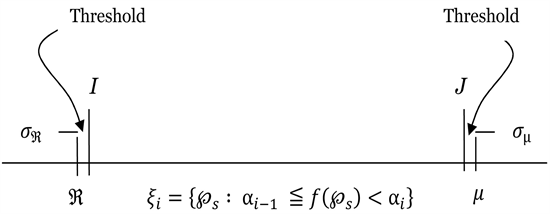
The boundaries of potential surprise in the economic decision provide a space between $\Re$ and μ such that intermediate point of $\Re$ and μ are Herbert Simon’s bounded (Katzner, 1986; Herbert, 1987; Kreeps, 2002) . We shall proceed by showing that the space of potential surprise bounding economic decision be a function $f\left({\wp }_s\right)$ and measurable in the interval $\left[\Re ,\mu \right]$ .

Lemma 1: If $E=E_1\cup E_2\cup \cdots$ where $E_1,E_2,\cdots$ are mutually disjointed, then,

${\displaystyle {\int }_{E}f\left(x\right)\text{d}x}={\displaystyle {\int }_{E_1}f\left(x\right)\text{d}x}+{\displaystyle {\int }_{E_2}f\left(x\right)\text{d}x}+\cdots$

Proof: If “S” is an upper sum related to any partition and “s” is also a lower sum related to same or different partition, then,

$S\ge I\ge J\ge s$ .

With I as the greatest lower bound of all upper sums, as a consequence, $S\ge I$ . Taking J as the least upper bound of all lower sums, as a consequence, $J\ge s$ . Corresponding, $I\ge J$ for the case of not mutually disjoint.

Complimentary,

${\displaystyle {\int }_{E}f\left(x\right)\text{d}x}={\displaystyle {\int }_{E_1}f\left(x\right)\text{d}x}+{\displaystyle {\int }_{E_2}f\left(x\right)\text{d}x}$ .

Holds for

$S\ge I\ge J\ge s$ .

Lemma 2: If $f\left(x\right)$ and $g\left(x\right)$ are bounded and measurable on E, and

${\displaystyle {\int }_E\left[f\left(x\right)+g\left(x\right)\right]\text{d}x}={\displaystyle {\int }_{E}f\left(x\right)\text{d}x}+{\displaystyle {\int }_{E}g\left(x\right)\text{d}x}$ .

Then $f\left(x\right)$ is Lebesque integrable if and only if for any $E>0$ there exist a partition with upper and lower sums $S,s$ for which $S-s<\epsilon$ .

Proof: In a Lebesgue metric space, if for $\epsilon >0$ there correspond a partition such that $S-s<E$ . Borrowing from Lemma 1, in which,

$S\ge I\ge J\ge s$ .

Then, $0\le I-J\le S-s<\epsilon$ .

Putting $I=J$ with $\epsilon$ as any arbitrary small gaps, then $f\left(x\right)$ is Lebesgue integrable. Conversely, for $I=J$ and if $\epsilon >0$ there exist a partition such that

$S<I+\frac{\epsilon }{2}$ .

Since $I=g.l.b$ of all upper sums and $s>J-\frac{\epsilon }{2}$ with $J=l.u.b$ of all lower

sums.

As a consequence,

$S-s<\left(I+\frac{\epsilon }{2}\right)-\left(J-\frac{\epsilon }{2}\right)=\epsilon$ .

Taking any two real outcome, say γ and Γ such that $\gamma <f\left({\wp }_s\right)<\Gamma$ , we can have γ and Γ as subextremes of $\Re$ and μ and slicing it into n-decision groups by taking such values as, ${\alpha }_1,{\alpha }_2,\cdots ,{\alpha }_{n-1}$ so that

$\gamma ={\alpha }_0<{\alpha }_1<{\alpha }_2<\cdots <{\alpha }_{n-1}=\Gamma$ .

Taking a particular set of sub decision group as a cluster of potential surprise and letting, ${\xi }_i,i=1,2,\cdots ,n$ the group of all ${\wp }_s$ in $\left[\Re ,\mu \right]$ so that ${\alpha }_{i-1}\le f\left({\wp }_s\right)<{\alpha }_i$ , then,

${\xi }_i=\left\{{\wp }_s:{\alpha }_{i-1}\le f\left({\wp }_s\right)<{\alpha }_i\right\}$ with $i=1,2,\cdots ,k$ (1)

Supposing all ${\xi }_i$ is quantifiable ( ${�}_e$ ) in “k”, for which,

${�}_e\left(k\right)\ge {�}_e\left(k\cap {\xi }_i\right)+{�}_e\left(k\cap {\bar{\xi }}_i\right)$

and are verified to be disjoint. Taking the upper and lower bounds in $\Re$ and μ as outcomes as awful/implausible and astounding/implausible limits, then.

$\{\begin{array}{l}{S}_{a/1}={\displaystyle {\sum }_{i=1}^n{\alpha }_i{�}_e}\left({\xi }_i\right):S_{a/1}=\text{Upperboundforawful}/\text{implausiblepossibility}\\ s_{a/2}={\displaystyle {\sum }_{i=1}^n{\alpha }_{i-1}{�}_e}\left({\xi }_i\right):s_{a/2}=\text{Lowerboundforastounding}/\text{implausiblepossibility}\end{array}$

By randomizing all sub-decision group in the cluster, limiting value, of I and J can be obtained for $S_{a/1}$ and $s_{a/2}$ taking I = greater lower bound of all values of $S_{a/1}$ for all sub-decision group J = least upper bound of all values of $s_{a/2}$ for all sub-decision group.

Taking the bounds of potential surprise in the bounds of the decision interval $\left[\Re ,\mu \right]$ with intermediate points as subjective decisions arrays limiting in I and J of [ $\Re$ and μ] we have that $S_{a/1}$ and $s_{a/2}$ being upper and lower sums corresponding to a sub-decision group λ, with ϕ and ψ as least upper and greater lower bonds of $f\left({\wp }_s\right)$ in $\left[\Re ,\mu \right]$ , there exist,

$\psi \left(\mu -\Re \right)\le s_{a/2}\le S_{a/1}\le \varphi \left(\mu -\Re \right)$ (2)

Using the nation $S_{a/1}={\varphi }_1\left({\wp }_{s_1}-{\wp }_{s_0}\right)+\cdots +{\varphi }_n\left({\wp }_{s_n}-{\wp }_{s_{n-1}}\right)={\displaystyle \sum {\varphi }_i\Delta {\wp }_{s_i}}$

$s_{a/2}={\psi }_1\left({\wp }_{s_1}-{\wp }_{s_0}\right)+\cdots +{\psi }_n\left({\wp }_{s_n}-{\wp }_{s_{n-1}}\right)={\displaystyle \sum {\psi }_i\Delta {\wp }_{s_i}}$

$S_{a/1}={\displaystyle \underset{i=1}{\overset{n}{\sum }}{\varphi }_i\Delta {\wp }_{s_i}},s_{a/2}={\displaystyle \underset{i=1}{\overset{n}{\sum }}{\psi }_i\Delta {\wp }_{s_i}}$ .

Given that $\psi \le {\psi }_i\le {\varphi }_i\le \varphi$ and on multiplicative operation on $\Delta {\wp }_{s_i}$ and summing over i from 1 to n, we have

$\left|{\displaystyle \underset{i=1}{\overset{n}{\sum }}\psi \Delta {\wp }_{s_i}}\le {\displaystyle \underset{i=1}{\overset{n}{\sum }}{\psi }_i\Delta {\wp }_{s_i}}\right|\le \left|{\displaystyle \underset{i=1}{\overset{n}{\sum }}{\varphi }_i\Delta {\wp }_{s_i}}\le {\displaystyle \underset{i=1}{\overset{n}{\sum }}\varphi \Delta {\wp }_{s_i}}\right|$

$\psi {\displaystyle \underset{i=1}{\overset{n}{\sum }}\Delta {\wp }_{s_i}}\le s_{a/2}\le S_{a/1}\le \varphi {\displaystyle \underset{i=1}{\overset{n}{\sum }}\Delta {\wp }_{s_i}}$ (3)

Showing equations (2) = (3) and following the existence of I and J for $S_{a/1}$ and $S_{a/2}$ of $f\left({\wp }_s\right)$ on the space of [ $\Re$ and μ] then

$I_{\left[S_{a/1}\right]}={\displaystyle {\int }_{\Re }^{\bar{\mu }}f\left({\wp }_s\right)\text{d}}\left({\wp }_s\right),J_{\left[s_{a/2}\right]}={\displaystyle {\int }_{\bar{\Re }}^{\mu }f\left({\wp }_s\right)\text{d}\left({\wp }_s\right)}$ .

For which $I_{\left[S_{a/1}\right]}\ne J_{\left[s_{a/2}\right]}=>f\left({\wp }_s\right)$ is Lebesgue measurable and integrable in $\left[\Re ,\mu \right]$ with a common value of

${\displaystyle {\int }_{\Re }^{\mu }f\left({\wp }_s\right)\text{d}\left({\wp }_s\right)}$ .

Since $f\left({\wp }_s\right)$ is bounded and quantifiable space in $\Re$ and μ, it follows specifically that ξ is a quantifiable sequence in $\left[\Re ,\mu \right]$ and as a property of lebesgue summation $f_n\left({\wp }_s\right)$ on ξ is:

${\displaystyle {\int }_{\xi }f\left({\wp }_s\right)\text{d}{\wp }_s}={\displaystyle {\int }_{\Re }^{\mu }g\left({\wp }_s\right)\text{d}{\wp }_s}$ .

With $g\left({\wp }_s\right)=\{\begin{array}{ll}f\left({\wp }_s\right)\hfill & \text{if}{\wp }_s\in \xi \hfill \\ 0\hfill & \text{if}{\wp }_s\notin \xi \hfill \end{array}$

For which according to the sequence space sums of the upper and lower values of $S_{a/1}$ and $s_{a/2}$ given,

${\xi }_i=\left\{{\wp }_s:{\wp }_s\in \xi ,{\alpha }_{i-1}\le f\left(\wp \right)<{\alpha }_i\right\}$

This reduces the expression above to $\xi =\left[\Re ,\mu \right]$ . With $\langle f_n\left(\wp \right)\rangle$ as sequence of functions quantifiable ( ${�}_{\text{e}}$ ) on ξ, and if $\varphi \left(S_{a/1}\right)$ = Least upper bound $f_n\left({\wp }_s\right)$ and $\psi \left(S_{a/2}\right)$ = greatest lower bound $f_n\left({\wp }_s\right)$ . The $\varphi \left(S_{a/1}\right)$ and $\psi \left(S_{a/2}\right)$

are quantifiable in ξ. Since $\varphi \left(S_{a/1}\right)=l.u.b\left\{f_n\left({\wp }_s\right)\right\}=l.u.b\left\{f_i\left({\wp }_s\right),f_2\left({\wp }_s\right),\cdots \right\}$ and taking $\psi \left(S_{a/2}\right)=g.l.b\left\{f_n\left({\wp }_s\right)\right\}=g.l.b\left\{f_i\left({\wp }_s\right),f_2\left({\wp }_s\right),\cdots \right\}$ , then

${�}_e\left[\varphi \left(S_{a/1}\right)\ge k\right]={\displaystyle \underset{i=1}{\overset{\alpha }{\cup }}{�}_e}\left[f_n\left({\wp }_s\right)\ge k\right]$ as a consequence from Equation (1) since a

Countable union of quantifiable potential surprises group is also quantifiable.

2.2. Potential Surprise Space

We have proposed that economic decisions are bounded in the interval of $\left[\Re ,\mu \right]$ and therein with intermediate point provide potential for surprise decision over time as alternative forgone within the sequence (Shackle, 1949; Carter, 2015; Kreeps 2002) . The sequence of events within the space suggests that possibilities are components of the potential surprise.

Lemma 3: Every convergent sequence is Cauchy sequence.

Proof: Given the sequence of real numbers ( $a_n$ ) converges to L. Therefore for

any $\epsilon >0$ , we obtain no such that $\left|a_p-l\right|<\frac{\epsilon }{2}$ for all $p>n_0$ .

And, $\left|a_p-l\right|$ for all $q>n_0$ .

Similarly, for both set absorptivity of $P>n_0$ and $q>n_0$ , we have

$\left|a_p-a_q\right|=\left|\left(a_p-l\right)+\left(l-a_q\right)\right|\le \left|a_p-l\right|+\left|l-a_q\right|<\frac{\epsilon }{2}+\frac{\epsilon }{2}=\epsilon$ .

If $f\left({\wp }_s\right)\to \left[\Re ,\mu \right]$ , the sequence of potential outcome, as surprises in the bounded space $\left[\Re ,\mu \right]$ with,

${\alpha }_{i-1}\le f\left({\wp }_s\right)<{\alpha }_i$ is the sequence of ξ, for which

${\xi }_i=\left\{{\wp }_s:{\alpha }_{i-1}\le f\left({\wp }_s\right)<{\alpha }_i\right\}$

That this sequence is bounded and convergent is shown by

${\xi }_i=\left|{\xi }_i-\xi +\xi \right|\le \left|{\xi }_i-\xi \right|+\left|\xi \right|$ .

And having a real positive number $�$ such that $\left|{\xi }_i\right|<q$ for all i. We introduce a limiting point $i_o$ that makes $\left|{\xi }_i-\xi \right|<\epsilon$ any positive number for all $i>i_o$ .

Hence, $\left|{\xi }_i\right|<\epsilon +\left|\xi \right|$ for all $i>i_o$ .

Correspondingly relate that $\left|{\xi }_i\right|<q$ for all i if $�$ is taken as one of the largest numbers ${\xi }_1,{\xi }_2,\cdots ,{\xi }_{io},\epsilon +\left|\xi \right|$ . The potential surprise outcome is obtainable from the set of sub decision in the interval of $\left[{\Re }_i,{\mu }_i\right]$ with $i=1,2,3,\cdots$ , Having ${\Re }_1\le {\Re }_i\le {\mu }_i\le {\mu }_1$ bounded and monotonically increasing and decreasing sequences converges to $\Re$ and μ.

To show that an exert surprise exist is to put $\Re$ = μ. This is done by making.

$\mu -\Re =\left(\mu -{\mu }_i\right)+\left({\mu }_i-{\Re }_i\right)+\left({\Re }_i-\Re \right)$

$\left|\mu -\Re \right|\le \left|\mu -{\mu }_i\right|+\left|{\mu }_i-{\Re }_i\right|+\left|{\Re }_i-\Re \right|$ (4)

At the condition ε > 0, we deterime $i_0\to i>i_0$ .

$\left|\mu -{\mu }_i\right|<\frac{\epsilon }{3},\left|{\mu }_i-{\Re }_i\right|<\frac{\epsilon }{3},\left|{\Re }_i-\Re \right|<\frac{\epsilon }{3}$

From (4) $\left|\mu -\Re \right|<\epsilon$ , with ε as any positive number, then μ − $\Re$ = 0, or $\Re$ = μ.

The potency and appeal of Shackle’s theory of potential surprise is laced with limitation critique economic decisions based on determinism and went ahead to propose innovation and surprise as a symptomatic response for indeterminacy (Basili & Zappia, 2009) . Such indeterminacy is bounded in the subjective space of surprise which time seems to validate for the decision taker (Shackle, 1968; Zongzhi, 2009) . Being not a laboratory science, economic science allude credence to subjective expectations with several national dimensions of past time (found memories), future time (expectations) and present time(decision). Resolving these dimensions with their associated indeterminacy is profoundly found in isolating decision variable and treating the competing past and future variables in simultaneity within potential surprise space (Carter, 2015) . The potential surprise space with avalanche of subjective and divergent thoughts is epistemically resolved in bounds of $\Re$ (awful and implausible outcome) and μ (astounding and implausible outcome). Within this bound which has semblance with Herbert Simon’s bound properties have been shown to have sequence of event outcomes between $S_{a/1}$ to $s_{a/2}$ to be potential for surprise along the sequence. With $\Re$ and μ showing characterization of conjugate properties, the sequence of subjective outcomes for potential surprise converging to a decision point ( ${\Omega }_D$ ) can be deductively obtained by given any $\epsilon >0$ , (ε = any positive number) in a sequence of potential surprise outcomes ( ${\xi }_i$ ) converging to decision point ( ${\Omega }_D$ ). We can get $k_o$ such that:

$\left|{\xi }_{\theta }-{\Omega }_D\right|<\frac{\epsilon }{2}\text{if}\text{all}\theta >k_o$ .

Also true for $\left|{\xi }_{\lambda }-{\Omega }_D\right|<\frac{\epsilon }{2}$ if all $\lambda =k_o$ .

For both conditions of $\theta >k_o$ and $\lambda =k_o$ and by means of factor difference

$\left|{\xi }_{\theta }-{\xi }_{\lambda }\right|=\left|\left({\xi }_{\theta }-{\Omega }_D\right)+\left({\Omega }_D-{\xi }_{\lambda }\right)\right|\le \left|{\xi }_{\theta }-{\Omega }_D\right|+\left|{\Omega }_D-{\xi }_{\lambda }\right|<\frac{\epsilon }{2}+\frac{\epsilon }{2}=\epsilon$

This shows that the sequence of ${\xi }_i=\left\{{\wp }_s:{\alpha }_{i-1}\le f\left({\wp }_s\right)<{\alpha }_i\right\}$ bounded by $\left[\Re ,\mu \right]$ in the functions of $f\left({\wp }_s\right)$ are Cauchy sequence by the conjugate limits of $\Re$ and μ.

If we interchange the bounds of the pool of potential surprise by resizing them as conjugate multiple, in the form $\left|\Re \right|\mu$ and $\left|\mu \right|\Re$ , then operating their products gives

$O\le \left(\left|\Re \right|\mu -\left|\mu \right|\Re \right)\cdot \left(\left|\Re \right|\mu -\left|\mu \right|\Re \right)$ .

And as can be seen reduces to:

$\left|\Re ,\mu \right|\le \left|\Re |\mu \right|$ (5)

Provided $\Re$ and μ are bounds linearly related.

2.3. Summary

Shackle’s Potential Surprise theory in economic science has not received the desired application in economic problems owing to the subjective reasoning demands required by the theory. The efforts to making it a computable science has witnessed birth of probability and set theory by multi-valued mapping approaches as seen in the works of Dempster (1967, 1968) . Shafer progressively, in Shafer (1976, 1979) and (1982) empirically by Fioretti (2001) provided evidence theory for the construction of coherent picture of reality from evidence in an individual’s mind yet laced with subjectivity of measurements in probability space for new possibilities. Fuzzy logic computable method was also introduced by Fioretti (2001) with inductive use of interval logics to represent extremums. In all of these efforts, none has shown promise of computable process save for subjective beliefs from set theories and non-deterministic methods based on probabilities. Consequently this paper theorizes the use of measure theory to offer computation of the Shackelian potential surprise in an attempt to providing the theory with a quantitifiable schema.

3. Research Method

This paper moved from theoretical conceptualization to use of abductive proof for the formalization of the measurability of potential surprise in economic analysis. The process commenced with a deep and extensive economic literature review to favour an identified gap of quantifying Shackle’s theory of potential surprise. It established the theoretical concord of the Shackelian bounds of $\Re$ and μ by theory of measures using the Lebesgue space to show symmetries with upperbound for awful/implausible possibility $\left|S_{a/1}\right|$ and lower bound for astounding/implausible possibility $\left|S_{a/2}\right|$ . Following such established relation, a potential surprise space was theorized to show that an exert surprise exist in a sequence of potential surprises ( ${\wp }_s$ ) in outcomes converging to a new deviated decision ( ${\Omega }_D$ ) within the bounds of $\Re$ and μ. It proceeded to proving that economic decisions are indeterminate arising from potential surprise as a Chaotic state space $H\left(\aleph \right)$ with properties randomly dispersed and normalized within the bounds of $\Re$ and μ. Showing that economic decisions are indeterminate in such chaotic state space was carried out by showing the deviations of $\Re$ and μ ( ${\sigma }_{\Re }^2$ , ${\sigma }_{\mu }^2$ ) are conjugated variables with symmetricity properties and can commute exclusively for $\left(\hat{\Re },\hat{\mu }\right)=i{H}_T$ to obtain a relation for indeterminacy on the bounds of $\Re$ and μ.

3.1. Indeterminancy of Economic Decisions

Economic thoughts in favour of attempts at extinguishing Shackle’s potential surprise theory in economic decision are profoundly calling for exclusion of perfect possible for the realization of Shackle’s zero potential surprise outcomes (Starmer, 1993; Smith, 1961) . But Shackle’s strong point is that Statisticians results are based on probabilities of frequentative outcomes that are exogenous to other human contingent subjective needs and preference which are root sources of potential surprise in economic decisions (Carter, 2015) . Shackle’s theory draws from the strength that economic decisions are purely unique and it is a function of a state of mind. This alludes indeterminacy to economic decisions and rather favours predictability of economic decision variables within some boundaries (Jaffray & Philippe, 1997) . Indeterminacy of economic decision is further favoured with theoretics of economic unexpected economic collapse. In recent times most economic decisions taken on the basis of strong statistical results and observed frequency are in awe of Covid-19 interference that took economic decisions in “potential surprise”. This is also evident with decision made in Ukraine and Russia arising from the infliction of “potential surprise” from the war against previous economic decisions made.

In foregoing review of indeterminacy of economic decisions as a result of possibility of potential surprise, this paper shall proceed to show that within the bounds of subjectively awful and implausible outcome ( $\Re$ ) and subjectively astounding implausible outcomes (μ) a series of potential surprise outcomes exists with indeterminate properties (Shackle, 1980, 1983; Jaffray & Philippe, 1997).

Potential theory

It is impossible to determine economic decisions outside the bound of $\Re$ and μ which act as potential surprise space in economic decisions.

Proof

Suppose we have bounded space in length ${\wp }_s\left[\Re ,\mu \right]$ given the geometric representation

Let ${\sigma }_{\Re },{\sigma }_{\mu }$ be outside of bound of ${\wp }_s\left[\Re ,\mu \right]$ such that ${\sigma }_{\Re },{\sigma }_{\mu }$ are deviated variables from the sequence with chaotic property randomly dispersed outside of ${\wp }_s$ space with dynamic time (Knudsen, 2000) index T as

$H\left(\aleph \right)\equiv \underset{T\to \infty }{\lim }\frac{1}{T}{H}_T\left({\wp }_s{}_1,{\wp }_{s_2},\cdots ,{\wp }_{s_T}\right)$

If the process normalizes in the bounds of $\Re$ , μ as a stationary sequence from threshold point acting.

With preceding conditional chaos ( $H^{*}$ ) to stationary property of sequences of ${\wp }_s$ in ${\xi }_{\lambda }$ as;

$H^{*}\left(\aleph \right)\equiv \underset{T\to \infty }{\lim }\frac{1}{T}{H}_T\left({\wp }_s{}_T|{\wp }_{s_{T-1}},{\wp }_{s_{T-2}},\cdots ,{\wp }_{s_1}\right)$

Then

$H\left(\aleph \right)=H^{*}\left(\aleph \right)=H_T\left({\wp }_{s_2}|{\wp }_{s_1}\right)\cdots H\left({\wp }_{s_T}|{\wp }_{s_{T-1}}\right)$

Taking average deviations from decision point ( ${\Omega }_o$ ) by one to one mapping points in $\Re$ and μ as ${\wp }_s$ , in which, ${}^{\Re }D{}_i={\Re }_i-{\Omega }_D$ and ${}^{\mu }D{}_j={\mu }_j-{\Omega }_D$ so

that ${\Re }_{i=1}$ and ${\mu }_{j=1}$ , gives $\frac{1}{2}\left({}^{\Re }D{}_{i=1}+{}^{\mu }D{}_{j=1}\right)={\wp }_{s_1}$ . With $H\left(\aleph \right)$ and $H^{*}(\; \aleph \; )$

(Golan, 2006) as space state normalization metrics, for boundary condition stationarity occurring at $\Re$ , μ boundaries, than we have the standard deviations of $\Re$ , μ been in chaos from decision point ( ${\Omega }_D$ ) as ${\sigma }_{\Re }$ , ${\sigma }_{\mu }$ conjugated variables. Therefore,

${\sigma }_{\Re }^2=\langle \left({\Omega }_D-{\langle {\Omega }_D\rangle }^2\right)\rangle =\langle {\Omega }_D^2\rangle -{\langle {\Omega }_D\rangle }^2$ (6)

With ${\sigma }_{\Re }^2$ as the average squared difference from the decision point ( Ω D )

within the sequence ( ${\xi }_i$ ) of expectations values ${\left(\hat{\Re }-\langle \hat{\Re }\rangle \right)}^2$ overtime (T) in

chaotic state normalization metrics ( $H_T^{\text{*}}$ ) having chaotic rate of dispersion from ${\Omega }_D$ as:

$H\left({\wp }_S\right)=\underset{T\to \infty }{\lim }\frac{H\left({\wp }_s^T\right)}{T},$

${\wp }_s$ been a consequence of time (T). Rewriting the Expression (6) above with expectation outcome plausibility, we have:

${\sigma }_{\Re }^2=\langle H_T^{*}|{\left(\hat{\Re }-\langle \hat{\Re }\rangle \right)}^2|H_T^{*}\rangle$

Having ${\Omega }_D$ in bounds of $\Re$ and μ on Herbert Simon bound, we set: $\omega =\left(\hat{\Re }-\langle \hat{\Re }\rangle \right){\xi }_i$ as ${\sigma }_{\Re }^2=\langle \omega |\omega \rangle$ at $\Re$ -bound, and for μ-bound, we set,

$\Lambda =\left(\hat{\mu }-\langle \hat{\mu }\rangle \right)H^{*}\text{as}{\sigma }_{\mu }^2=\langle \Lambda |\Lambda \rangle$

Recalling expression (5) and substituting for ${\sigma }_{\Re }^2$ and ${\sigma }_{\mu }^2$ above we have

${\sigma }_{\Re }^2{\sigma }_{\mu }^2=\langle \omega |\omega \rangle \langle \Lambda |\Lambda \rangle \le {\left|\langle \omega |\omega \rangle \right|}^2$ (7)

Obtaining expression for (7) in their potential surprise values gives,

$\begin{array}{c}\langle \omega |\Lambda \rangle =\langle \left(\hat{\Re }-\langle \hat{\Re }\rangle \right)H_T^{*}|\left(\hat{\mu }-\langle \hat{\mu }\rangle \right)H_T^{*}\rangle \\ =\langle H_T^{*}\left(\hat{\Re }-\langle \hat{\Re }\rangle \right)\left(\hat{\mu }-\langle \hat{\mu }\rangle \right)H_T^{*}\rangle \\ =\langle H_T^{*}|\hat{\Re }\hat{\mu }{H}_T^{*}\rangle -\langle \mu \rangle \langle H_T^{*}|\hat{\Re }{H}_T^{*}\rangle -\langle \Re \rangle \langle H_T^{*}|\hat{\mu }{H}_T^{*}\rangle +\langle \Re \rangle \langle \mu \rangle \langle H_T^{*}|H_T^{*}\rangle \\ =\langle \hat{\Re }\hat{\mu }\rangle -\langle \hat{\mu }\rangle \langle \hat{\Re }\rangle \end{array}$

And by deploying the conjugate of $\langle \omega |\Lambda \rangle$ as test of symmetricity property we obtain

$\langle \Lambda |\omega \rangle =\langle \hat{\mu }\hat{\Re }\rangle -\langle \hat{\Re }\rangle \langle \hat{\mu }\rangle$

By standardizing the expression with complex number property of

$Z^{\text{*}}Z\ge {\left[\frac{1}{2_i}\left(Z-Z^{\text{*}}\right)\right]}^2$

Then $\langle \omega |\Lambda \rangle$ is substituted by Z and $Z^{*}$ for $\langle \Lambda |\omega \rangle$ to give,

$\begin{array}{c}{\sigma }_{\Re }^2{\sigma }_{\mu }^2\ge {\left[\frac{1}{2_i}\left(\langle \omega |\Lambda \rangle -\langle \Lambda |\omega \rangle \right)\right]}^2\\ \ge {\left[\frac{1}{2_i}\left(\langle \hat{\Re }\hat{\mu }\rangle -\langle \hat{\mu }\rangle \langle \hat{\Re }\rangle -\langle \hat{\mu }\hat{\Re }\rangle -\langle \hat{\Re }\rangle \langle \hat{\mu }\rangle \right)\right]}^2\end{array}$

This reduces to:

$\ge {\left|\frac{1}{2_i}\langle \left|\hat{\Re },\hat{\mu }\right|\rangle \right|}^2$

If $\hat{\Re }$ and $\hat{\mu }$ in symmetricity commute exclusively, then $\left[\hat{\Re }\hat{\mu }\right]=i{H}_T^{*}$ and by obtaining the square root of both sides, we have the indeterminacy expression for economic decision within the bounds of $\Re |\mu$ as

${\sigma }_{\Re }{\sigma }_{\mu }\ge \frac{H_T^{*}}{2}\text{or}\frac{1}{2}{H}_T^{*},$ (8)

$H_T^{*}$ been an Arbitrary chaotic economic state wherein T is the dynamic time of the process (Knudsen, 2000) for the expression in (8) suggests that economic decisions are bounded with surprises between an awful/implausible possibility ( $\Re$ ) and astounding/implausible possibility (μ). Between $\Re$ and μ presents us with ocean of potential surprises with indeterminate propensities. Implying that economic decisions cannot make outcome of both awful and astounding possibilities. If economic decisions is awful, then the astounding outcomes exists potentially and conjugatively if economic decisions is astounding, then an awful outcome exists potentially outcome exists potentially.

3.2. Analysis and Discussion

Drawing from the notion that information for economic decision are not finite (see Golan pg. 17/18) and shows spurious estimates over frequentative based probability outcomes, a tendency for entropy state (H) decisions arises with uncertainty outlook harping on the unpredictability expounded by the Shackelian

space, ${\sigma }_{\Re }{\sigma }_{\mu }=\frac{1}{H_T^{*}}$ .

In the light of such infinite propensities for economic outcomes from a probability dependent criterion, uncertainty therefore supports the state of indeterminacy from an entropic ( $H_T<\aleph$ ) information. This is especially the case when a decision maker knowledge or information catches is alien to the underlying characteristics behaviour of economic systems metric which often times induces entropy state from Zbili & Rama (2021) for a potential surprise as

$H=-{\langle \underset{i}{{\displaystyle \sum }}P{\left(x_i\right)}_T\ast {\log }_{2}P{\left(x_i\right)}_T\rangle }_T$ (9)

In the real sense of information and entropy, no economic decision is absolute and free of economic skews or moments from a mortal economic force of imbalances and future occurences. This was the mind of G.L.S Shackle and it is overt to say that decision space in economics are not turbulence (entropy) free and are characterized by indeterminate state from incomplete reasoning that births potential surprise.

For example, decision for housing investment predicated on the developer’s budget based on certain economic decision metrics, as IRR, ARR, NPV, UNACOST, capitalized cost, etc. can as a matter of incomplete information be compelled to succumb to mortal economic force of indeterminacy. Suppose the developer above was foreclosed to other economic restraint in guiding his decisions, such outliers are deemed to be subjective ignorance to the decision maker, but yet governed by the information of the decision space with entropic probability attributes

$H\left(p\right)={\displaystyle \underset{i=1}{\overset{m}{\sum }}{P}_i{\log }_2\frac{1}{P_i}}$ (10)

which does not rely on distinct realized randomized variables, $x_1,x_2,x_3,\cdots ,x_m$ but on their probabilities, $x_1|p_1,x_2|p_2,x_3|p_3,\cdots ,x_m|p_m$ . In our accompanying analysis below, we shall proceed to map decision metrics indices for a potential developer say IRR to a probability enabled entropy state computation as congruent parameters to obtaining the limit state of the developers economic decision. Based on computational advice from the developer’s budget, the developer obtains five (5) consecutive IRR for five (5) alternatives of housing A or B. on the basis of joint entropy dependence, we associate their probabilities as:

$P\left(A|B\right)$ , letting $P\left(A=a_i\right)=P_i$ , $P\left(B=b_j\right)=P_j$ then,

$P\left(A=a_i,B=b_j\right)={\lambda }_{ij},P\left(A|B\right)=P\left(A=a_i|B=b_j\right)=P_{i|j}$

By commutating the probability values, we have $P\left(A|B\right),P\left(B|A\right)$ implying $P\left(B|A\right)=P\left(B=b_j|A=a_i\right)=q_{j|i}$ for which

$P_i={\displaystyle {\sum }_{i=1}^i{X}_{ij}},q_i={\displaystyle {\sum }_{j=1}^j{\lambda }_{ji}}$

Then joint entropy of A and B given:

$H\left(A|B\right)=\underset{ij}{{\displaystyle \sum }}{\lambda }_{ij}\log \frac{1}{{\lambda }_{ij}}=-\underset{ij}{{\displaystyle \sum }}{\lambda }_{ij}\log {\lambda }_{ij}$

On a more general note, entropy (Chernoff forms with α-) has been written for processes with incomplete random variable by Renyi (1970) with order α- as

$H_{\alpha }^R\left(p\right)=\frac{1}{1-\alpha }\log \underset{k}{{\displaystyle \sum }}{P}_k^{\alpha }$ (11)

Cross entropy between distributions as mentioned in Golan (2006) by Renyi (1970) for difference between two distributions, p and q of order α- was given as:

$D_{\alpha }^R\left(x|y\right)=D_{\alpha }^R\left(p\left|\right|q\right)=\frac{1}{1-\alpha }\log \underset{k}{{\displaystyle \sum }}\frac{P_k^{\alpha }}{q_k^{\alpha -1}}$ (12)

Construction economics investigation for a prospective developer with five housing alternative to decide from on the basis of budget returned advise of IRR having two scenarios of flat (or continuous IRR) or discontinued IRR on the five alternative investment are presented (see Table 1).

Lower entropy from the first scenario in Table 2 shows that investment decision in scenario is more realistic with less ignorance. However, according to G.L.S Shackles potential surprise theory, espitemic knowledge is bounded between lower and higher entropy beyond which the investment decision is indeterminate.

Table 1. Information and entropy values for investment decisions.

Table 2. Information and probability.

Ever since, Renyi (1970) work, there has been a systematic bibliography on generalized entropy reviewed in Golan (2006) for Cressie & Read (1984) and particularly by Tsallis (1988) as,

$D_{\alpha }^T\left(x|y\right)=D_{\alpha }^T\left(p\left|\right|q\right)=\frac{1}{1-\alpha }\left(\underset{k}{{\displaystyle \sum }}\frac{P_k^{\alpha }}{q_k^{\alpha -1}}-1\right)$ (13)

Renyi (1970) and Tsallis (1988) entropies have been harmonized as stated in Golan (2006) in Tsallis (1988) and Holste et al. (1998) to be of the form;

$H_{\alpha }^R\left(x\right)=\frac{1}{1-\alpha }\log \left[1+\left(1-\alpha \right)\log H_{\alpha }^T\right]$ (14)

By connecting Renyi (1970) , Tsallis (1988) and Holste et al. (1998) , Golan (2006) reported in Golan (2002) as stringing the three form of entropies, this form as:

$D_{\alpha +1}^R\left(p\left|\right|q\right)=-\frac{1}{\alpha }\log \left[1-\alpha D_{\alpha +1}^T\left(p\left|\right|q\right)\right]$ (15)

For emphasis, over potential surprise space ( ${\wp }_s$ ) with chaos (entropy) properly will continue to be denoted with $H_T$ for a function of indeterminacy from incomplete reasoning (information) owing to the stochastic property of the space.

4. Conclusion

This paper provided validation of potential surprise theory as a contribution to economics literature. It moved from highlighting the misconception of the theory amongst 21st century economists who had reservations for the theory arising from its subjective approach rather than robust mathematical and computable approach. Following the foundation of incomplete knowledge theory mathematical background, a theoretical build up was argued for, in support of potential surprise in economic decision. It moved from a conjecture of potential surprise space which hitherto has been proposed according to its theory to be bounded by two parameters of $\Re$ (for subjectively awful and implausible outcome) and μ (for subjectively astounding and implausible outcome). Analytic space duality showed that extremums exist between $\Re$ and μ as bounded variation limits with sequence outcomes possessing propensity for potential surprises from a decision point. Following the chaotic behavior propensities of potential surprise variables, deviations from the bounds of $\Re$ and μ in their standard forms were manipulatively treated as inequalities being conjugate by the theory of potential surprise as impossible to simultaneously obtain $\Re$ and μ in economic decision. As a consequence of the proof, it became apparent that economic decisions are limited to indeterminacy from the occurrence of both $\Re$ and μ in a chaotically abductive process showing potential for surprise.

Statements and Declarations

This paper has no accruing financial interest or had any grant that is directly or indirectly related to the work submitted for publication.

Competing Interest

We hereby declare that this paper and the efforts of putting it together have no known competing financial/other interests or personal relationships that could have appeared to influence the research work reported in this paper.

References

1. 1. Basili, M., & Zappia, C. (2009). Shackle and Modern Decision Theory. Metroeconomica, 60, 245-282. https://doi.org/10.1111/j.1467-999X.2008.00333.x [Paper reference 1]


2. 2. Bayes, T., & Price, R. (1763). An Essay towards Solving a Problem in the Doctrine of Chances. In E. S. Pearson, & M. G. Kendall (Eds.), Reprinted in Studies in the History of Statistics and Probability (pp. 134-153). Griffin. [Paper reference 1]


3. 3. Cantillo, A. F. (2015). Shackle’s Potential Surprise Function and the Formation of Expectations in a Monetary Economy. Journal of Post Keynesian Economics, 37, 233-253. [Paper reference 2]


4. 4. Carter, C. F. (2015). Time in Economics. The Economic Journal, 68, 543-545. https://doi.org/10.2307/2227561 [Paper reference 6]


5. 5. Chermack, T. J. (2004). A Theoretical Model of Scenario Planning. Human Resource Development Review, 3, 301-325. https://doi.org/10.1177/1534484304270637 [Paper reference 1]


6. 6. Cressie, N., & Read, T. R. C. (1984). Multinomial Goodness of Fit Tests. Journal of Royal Statistical Society B, 46, 440-464. https://doi.org/10.1111/j.2517-6161.1984.tb01318.x [Paper reference 1]


7. 7. Dempster, A. O. (1967). Upper and Lower Probabilities Induced by a Multivalued Mapping. The Annals of Mathematical Statistics, 38, 325-338. https://doi.org/10.1214/aoms/1177698950 [Paper reference 2]


8. 8. Dempster, A. P. (1968). A Generalization of Bayesian Inference. Journal of the Royal Statistical Society B, 30, 205-247. https://doi.org/10.1111/j.2517-6161.1968.tb00722.x


9. 9. Derbyshire, J. (2017). Potential Surprise Theory as a Theoretical Foundation for Scenario Planning. Technological Forecasting and Social Change, 124, 77-87. https://doi.org/10.1016/j.techfore.2016.05.008 [Paper reference 1]


10. 10. Dubois, D., & Prade, H. (1988). Possibility Theory. Plenum Press. [Paper reference 1]


11. 11. Dunn, S. (2001). Bounded Rationality Is Not Fundamental Uncertainty: A Post-Keynesian Perspective (33 p.). Staffordshire University. [Paper reference 1]


12. 12. Dunn, S. (2002). Keynes, Uncertainty and the Competitive Process (40 p.). Staffordshire University. [Paper reference 1]


13. 13. Ewens, W. J. (1990). The Sampling Theory of Selectively Neutral Alleles. Theoretical Population Biology, 3, 87-112. https://doi.org/10.1016/0040-5809(72)90035-4 [Paper reference 1]


14. 14. Fioretti, G. (2001). A Mathematical Theory of Evidence for G.L.S, Shackle. Mind & Society, 3, 77-98. https://doi.org/10.1007/BF02512076 [Paper reference 6]


15. 15. Ford, J. (2001). Shackle’s Theory of Decision Making under Uncertainty: Synopsis and Brief Appraisal. Journal of Economic Studies, 12, 49-69. https://doi.org/10.1108/eb002594 [Paper reference 1]


16. 16. Ford, J. L., & Ghose, S. (1994). Belief, Credibility, Disbelief, Possibility, Potential Surprise and Probability as Measures of Uncertainty: Some Experimental Evidence. Discussion Paper No. 94-22, University of Birmingham, Department of Economics. [Paper reference 1]


17. 17. Ford, J. L., & Ghose, S. (1995). Shackle’s Theory of Decisions-Making under Uncertainty: The Findings of a Laboratory Experiments. Discussion Paper No. 95-08, University of Birmingham, Department of Economics. [Paper reference 1]


18. 18. Gilboa, I., & Schmeidler, D. (1993). Updating Ambiguous Beliefs. Journal of Economic Theory, 59, 33-49. https://doi.org/10.1006/jeth.1993.1003 [Paper reference 1]


19. 19. Golan, A. (2002). Information and Entropy Econometrics-Editors View. Journal of Econometrics, 107, 1-15. https://doi.org/10.1016/S0304-4076(01)00110-5 [Paper reference 1]


20. 20. Golan, A. (2006). Information and Entropy Econometrics—A Review and Synthesis. Foundations and Trends in Econometrics, 2, 1-145. https://doi.org/10.1561/0800000004 [Paper reference 5]


21. 21. Hargreaves-Heap, S., & Hollis, M. (1987). Determinism. In The New Palgrave: A Dictionary of Economics (pp. 816-818). Macmillan. https://doi.org/10.1057/978-1-349-95121-5_582-1 [Paper reference 1]


22. 22. Herbert, S. (1987). Bounded Rationality. In M. N. Eatwell (Ed.), The New Palgrave: A Dictionary of Economics (Vol. 1 p. 266-267). Macmillan. [Paper reference 1]


23. 23. Holste, D., Grobe, I., & Herzel, H. (1998). Bayes’ Estimators of Generalized Entropies. Journal of Physics A: Mathematical and General, 31, 2551-2566. https://doi.org/10.1088/0305-4470/31/11/007 [Paper reference 2]


24. 24. Hoppe, F. M. (1987). The Sampling Theory of Neutral Alleles and Urn Model in Population Genetics. Journal of Mathematical Biology, 25, 123-159. https://doi.org/10.1007/BF00276386 [Paper reference 1]


25. 25. Jaffray, J. Y. (1989). Linear Utility Theory for Belief Functions. Operations Research Letters, 8, 107-112. https://doi.org/10.1016/0167-6377(89)90010-2 [Paper reference 2]


26. 26. Jaffray, J. Y. (1992). Bayesian Updating and Belief Functions. IEEE Transactions on Systems, Man and Cybernetics, 22, 1144-1152. https://doi.org/10.1109/21.179852 [Paper reference 1]


27. 27. Jaffray, J. Y., & Philippe, F. (1997). On the Existence of Subjective Upper and Lower Probabilities. Mathematics of Operations Research, 22, 165-185. https://doi.org/10.1287/moor.22.1.165 [Paper reference 2]


28. 28. Jens, C. E. (2017). Political Uncertainty and Investment: Causal Evidence from U.S. Gubernatorial Elections. Journal of Financial Economics, 124, 563-579. https://doi.org/10.1016/j.jfineco.2016.01.034 [Paper reference 1]


29. 29. Katzner, D. W. (1986). Potential Surprise, Potential Confirmation, and Probability. Journal of Post-Keynesian Economics, 9, 58-78. https://doi.org/10.1080/01603477.1986.11489600 [Paper reference 2]


30. 30. Klir, G. J., & Harmanec, D. (1994). On Modal Logic Interpretation of Possibility Theory. International Journal of Uncertainty, Fuzziness and Knowledge-Based Systems, 2, 237-245. https://doi.org/10.1142/S0218488594000183 [Paper reference 1]


31. 31. Knudsen, T. (2000). Dynamic Time and Originative Choice. In Critical Realism Reunion Conference (27 p.). University of Southern Denmark, Odense University. [Paper reference 2]


32. 32. Kreeps, D. (2002). Bounded Rationality. In P. Newman (Ed.), The New Palgrave Dictionary of Economics and the Law (Vol. 1, pp. 168-173). Macmillan. https://doi.org/10.1007/978-1-349-74173-1_37 [Paper reference 2]


33. 33. Laplace, P. S. (1814). Essai philosophique sur les probabilités. Courcier. [Paper reference 1]


34. 34. Loasby, B. (2011). Uncertainty and Imagination, Illusion and Order: Shackleian Connections. Cambridge Journal of Economics, 35, 771-783. https://doi.org/10.1093/cje/beq048 [Paper reference 1]


35. 35. Ponsonnet, J. M. (1996). The Best and the Worst in G.L.S. Shackle’s Decision Theory. Uncertainty in Economic Thought. [Paper reference 1]


36. 36. Radner, R. (1987). Uncertainty and General Equilibrium. In M. N. Eatwell (Ed.), The New Palgrave: A Dictionary of Economics (Vol. 4, pp. 738-741). Macmillan. [Paper reference 1]


37. 37. Ramirez, R., & Selin, C. (2014). Plausibility and Probability in Scenario Planning. Foresight, 16, 54-74. https://doi.org/10.1108/FS-08-2012-0061 [Paper reference 1]


38. 38. Renyi, A. (1970). Probability Theory. North-Holland. [Paper reference 5]


39. 39. Resconi, G., Klir, G. J., & St. Clair, U. (1992). Hierarchical Uncertainty Metatheory Based upon Modal Logic. International Journal of General Systems, 21, 23-50. https://doi.org/10.1080/03081079208945051 [Paper reference 1]


40. 40. Sargent, T. (1987). Rational Expectations. In M. N. Eatwell (Ed.), The New Palgrave: A Dictionary of Economics (Vol. 4, pp. 76-79). Macmillan. [Paper reference 1]


41. 41. Shackle, G. L. S. (1949). Expectation in Economics. Cambridge University Press. [Paper reference 2]


42. 42. Shackle, G. L. S. (1968). Expectations Investment and Income. Oxford University Press. [Paper reference 1]


43. 43. Shackle, G. L. S. (1976). Epistemics and Economics. Cambridge University Press. [Paper reference 1]


44. 44. Shackle, G. L. S. (1980). Imagination, Unknowledge and Choice. Greek Economic Review, 2, 95-110. [Paper reference 1]


45. 45. Shackle, G. L. S. (1982). Time and the Structure of Economic Analysis: Comment. Journal of Post-Keynesian Economics, 5, 180-181. https://doi.org/10.1080/01603477.1982.11489354 [Paper reference 1]


46. 46. Shackle, G. L. S. (1983). The Bounds of Unknowledge. In J. Wiseman (Ed.), Beyond Positive Economics? Proceedings of Section F (Economics) of the British Association for the Advancement of Science, York 1981 (pp. 2-37). Macmillan. https://doi.org/10.1007/978-1-349-16992-4_3 [Paper reference 1]


47. 47. Shafer, G. (1976). A Mathematical Theory of Evidence. Princeton University Press. https://doi.org/10.1515/9780691214696 [Paper reference 3]


48. 48. Shafer, G. (1979). Allocations of Probability. Annals of Probability, 7, 827-839. https://doi.org/10.1214/aop/1176994941


49. 49. Shafer, G. (1982). Belief Functions and Parametric Models. Journal of the Royal Statistical Society B, 44, 322-352. https://doi.org/10.1111/j.2517-6161.1982.tb01211.x [Paper reference 2]


50. 50. Shafer, G. (1986). The Combination of Evidence. International Journal of Intelligent Systems, 1, 155-179. https://doi.org/10.1002/int.4550010302 [Paper reference 1]


51. 51. Shafer, G. (1990). Perspectives on the Theory and Practices of Belief Functions. International Journal of Approximate Reasoning, 4, 323-362. https://doi.org/10.1016/0888-613X(90)90012-Q [Paper reference 1]


52. 52. Smith, C. A. B. (1961). Consistency in Statistical Inference and Decision. Journal of the Royal Statistical Society B, 23, 1-25. https://doi.org/10.1111/j.2517-6161.1961.tb00388.x [Paper reference 1]


53. 53. Starmer, C. (1993). The Psychology of Uncertainty in Economic Theory: A Critical Appraisal and a Fresh Approach. Review of Political Economy, 5, 181-196. https://doi.org/10.1080/09538259300000013 [Paper reference 1]


54. 54. Tsallis, C. (1988). Possible Generalization of Baltzman-Gibbs Statistics. Journal of Statistical Physics, 52, 479. https://doi.org/10.1007/BF01016429 [Paper reference 4]


55. 55. Williams, P. M. (1976). Indeterminate Probabilities. In M. Przelecki, K. Szianiawaski, & R. W6jcîcki (Eds.), Formal Methods in the Methodology of Empirical Sciences (pp. 229-246). D. Reidel Publishing Company. https://doi.org/10.1007/978-94-010-1135-8_16 [Paper reference 1]


56. 56. Wiseman, J. (1983). The Bounds of Unknowledge. In J. Wiseman (Ed.), Beyond Positive Economics (pp. 28-37). St. Martin’s Press. https://doi.org/10.1007/978-1-349-16992-4 [Paper reference 1]


57. 57. Wright, G., & Goodwin, P. (2009). Decision Making and Planning under Low Levels of Predictability: Enhancing the Scenario Method. International Journal of Forecasting, 25, 813-825. https://doi.org/10.1016/j.ijforecast.2009.05.019 [Paper reference 1]


58. 58. Zabell, S. L. (1992). Predicting the Unpredictable. Synthese, 90, 205, 232. https://doi.org/10.1007/BF00485351 [Paper reference 2]


59. 59. Zbili, M., & Rama, S. (2021). A Quick and Easy Way to Estimate Entropy and Mutual Information for Neuroscience. Frontiers in Neuroinformatics, 15, Article ID: 596443. https://doi.org/10.3389/fninf [Paper reference 1]


60. 60. Zhang, F., Xu, Z. Y., & Huang, H. Q. (2022). Policy Swings of a Centralized Government: A Dynamic Optimizing Decision-Making Model and a Case of China. Modern Economy, 13, 566-579. https://doi.org/10.4236/me.2022.134030 [Paper reference 1]


61. 61. Zongzhi, L. A. (2009). Application of Shackle’s Model and System Optimization for Highway Investment Decision Making under Uncertainty. Journal of Transport Engineering, 135, 129-139. https://doi.org/10.1061/(ASCE)0733-947X(2009)135:3(129) [Paper reference 1]

Conflicts of Interest

The authors declare no conflicts of interest regarding the publication of this paper.

References

[1]	Basili, M., & Zappia, C. (2009). Shackle and Modern Decision Theory. Metroeconomica, 60, 245-282. https://doi.org/10.1111/j.1467-999X.2008.00333.x
[2]	Bayes, T., & Price, R. (1763). An Essay towards Solving a Problem in the Doctrine of Chances. In E. S. Pearson, & M. G. Kendall (Eds.), Reprinted in Studies in the History of Statistics and Probability (pp. 134-153). Griffin.
[3]	Cantillo, A. F. (2015). Shackle’s Potential Surprise Function and the Formation of Expectations in a Monetary Economy. Journal of Post Keynesian Economics, 37, 233-253.
[4]	Carter, C. F. (2015). Time in Economics. The Economic Journal, 68, 543-545. https://doi.org/10.2307/2227561
[5]	Chermack, T. J. (2004). A Theoretical Model of Scenario Planning. Human Resource Development Review, 3, 301-325. https://doi.org/10.1177/1534484304270637
[6]	Cressie, N., & Read, T. R. C. (1984). Multinomial Goodness of Fit Tests. Journal of Royal Statistical Society B, 46, 440-464. https://doi.org/10.1111/j.2517-6161.1984.tb01318.x
[7]	Dempster, A. O. (1967). Upper and Lower Probabilities Induced by a Multivalued Mapping. The Annals of Mathematical Statistics, 38, 325-338. https://doi.org/10.1214/aoms/1177698950
[8]	Dempster, A. P. (1968). A Generalization of Bayesian Inference. Journal of the Royal Statistical Society B, 30, 205-247. https://doi.org/10.1111/j.2517-6161.1968.tb00722.x
[9]	Derbyshire, J. (2017). Potential Surprise Theory as a Theoretical Foundation for Scenario Planning. Technological Forecasting and Social Change, 124, 77-87. https://doi.org/10.1016/j.techfore.2016.05.008
[10]	Dubois, D., & Prade, H. (1988). Possibility Theory. Plenum Press.
[11]	Dunn, S. (2001). Bounded Rationality Is Not Fundamental Uncertainty: A Post-Keynesian Perspective (33 p.). Staffordshire University.
[12]	Dunn, S. (2002). Keynes, Uncertainty and the Competitive Process (40 p.). Staffordshire University.
[13]	Ewens, W. J. (1990). The Sampling Theory of Selectively Neutral Alleles. Theoretical Population Biology, 3, 87-112. https://doi.org/10.1016/0040-5809(72)90035-4
[14]	Fioretti, G. (2001). A Mathematical Theory of Evidence for G.L.S, Shackle. Mind & Society, 3, 77-98. https://doi.org/10.1007/BF02512076
[15]	Ford, J. (2001). Shackle’s Theory of Decision Making under Uncertainty: Synopsis and Brief Appraisal. Journal of Economic Studies, 12, 49-69. https://doi.org/10.1108/eb002594
[16]	Ford, J. L., & Ghose, S. (1994). Belief, Credibility, Disbelief, Possibility, Potential Surprise and Probability as Measures of Uncertainty: Some Experimental Evidence. Discussion Paper No. 94-22, University of Birmingham, Department of Economics.
[17]	Ford, J. L., & Ghose, S. (1995). Shackle’s Theory of Decisions-Making under Uncertainty: The Findings of a Laboratory Experiments. Discussion Paper No. 95-08, University of Birmingham, Department of Economics.
[18]	Gilboa, I., & Schmeidler, D. (1993). Updating Ambiguous Beliefs. Journal of Economic Theory, 59, 33-49. https://doi.org/10.1006/jeth.1993.1003
[19]	Golan, A. (2002). Information and Entropy Econometrics-Editors View. Journal of Econometrics, 107, 1-15. https://doi.org/10.1016/S0304-4076(01)00110-5
[20]	Golan, A. (2006). Information and Entropy Econometrics—A Review and Synthesis. Foundations and Trends in Econometrics, 2, 1-145. https://doi.org/10.1561/0800000004
[21]	Hargreaves-Heap, S., & Hollis, M. (1987). Determinism. In The New Palgrave: A Dictionary of Economics (pp. 816-818). Macmillan. https://doi.org/10.1057/978-1-349-95121-5_582-1
[22]	Herbert, S. (1987). Bounded Rationality. In M. N. Eatwell (Ed.), The New Palgrave: A Dictionary of Economics (Vol. 1 p. 266-267). Macmillan.
[23]	Holste, D., Grobe, I., & Herzel, H. (1998). Bayes’ Estimators of Generalized Entropies. Journal of Physics A: Mathematical and General, 31, 2551-2566. https://doi.org/10.1088/0305-4470/31/11/007
[24]	Hoppe, F. M. (1987). The Sampling Theory of Neutral Alleles and Urn Model in Population Genetics. Journal of Mathematical Biology, 25, 123-159. https://doi.org/10.1007/BF00276386
[25]	Jaffray, J. Y. (1989). Linear Utility Theory for Belief Functions. Operations Research Letters, 8, 107-112. https://doi.org/10.1016/0167-6377(89)90010-2
[26]	Jaffray, J. Y. (1992). Bayesian Updating and Belief Functions. IEEE Transactions on Systems, Man and Cybernetics, 22, 1144-1152. https://doi.org/10.1109/21.179852
[27]	Jaffray, J. Y., & Philippe, F. (1997). On the Existence of Subjective Upper and Lower Probabilities. Mathematics of Operations Research, 22, 165-185. https://doi.org/10.1287/moor.22.1.165
[28]	Jens, C. E. (2017). Political Uncertainty and Investment: Causal Evidence from U.S. Gubernatorial Elections. Journal of Financial Economics, 124, 563-579. https://doi.org/10.1016/j.jfineco.2016.01.034
[29]	Katzner, D. W. (1986). Potential Surprise, Potential Confirmation, and Probability. Journal of Post-Keynesian Economics, 9, 58-78. https://doi.org/10.1080/01603477.1986.11489600
[30]	Klir, G. J., & Harmanec, D. (1994). On Modal Logic Interpretation of Possibility Theory. International Journal of Uncertainty, Fuzziness and Knowledge-Based Systems, 2, 237-245. https://doi.org/10.1142/S0218488594000183
[31]	Knudsen, T. (2000). Dynamic Time and Originative Choice. In Critical Realism Reunion Conference (27 p.). University of Southern Denmark, Odense University.
[32]	Kreeps, D. (2002). Bounded Rationality. In P. Newman (Ed.), The New Palgrave Dictionary of Economics and the Law (Vol. 1, pp. 168-173). Macmillan. https://doi.org/10.1007/978-1-349-74173-1_37
[33]	Laplace, P. S. (1814). Essai philosophique sur les probabilités. Courcier.
[34]	Loasby, B. (2011). Uncertainty and Imagination, Illusion and Order: Shackleian Connections. Cambridge Journal of Economics, 35, 771-783. https://doi.org/10.1093/cje/beq048
[35]	Ponsonnet, J. M. (1996). The Best and the Worst in G.L.S. Shackle’s Decision Theory. Uncertainty in Economic Thought.
[36]	Radner, R. (1987). Uncertainty and General Equilibrium. In M. N. Eatwell (Ed.), The New Palgrave: A Dictionary of Economics (Vol. 4, pp. 738-741). Macmillan.
[37]	Ramirez, R., & Selin, C. (2014). Plausibility and Probability in Scenario Planning. Foresight, 16, 54-74. https://doi.org/10.1108/FS-08-2012-0061
[38]	Renyi, A. (1970). Probability Theory. North-Holland.
[39]	Resconi, G., Klir, G. J., & St. Clair, U. (1992). Hierarchical Uncertainty Metatheory Based upon Modal Logic. International Journal of General Systems, 21, 23-50. https://doi.org/10.1080/03081079208945051
[40]	Sargent, T. (1987). Rational Expectations. In M. N. Eatwell (Ed.), The New Palgrave: A Dictionary of Economics (Vol. 4, pp. 76-79). Macmillan.
[41]	Shackle, G. L. S. (1949). Expectation in Economics. Cambridge University Press.
[42]	Shackle, G. L. S. (1968). Expectations Investment and Income. Oxford University Press.
[43]	Shackle, G. L. S. (1976). Epistemics and Economics. Cambridge University Press.
[44]	Shackle, G. L. S. (1980). Imagination, Unknowledge and Choice. Greek Economic Review, 2, 95-110.
[45]	Shackle, G. L. S. (1982). Time and the Structure of Economic Analysis: Comment. Journal of Post-Keynesian Economics, 5, 180-181. https://doi.org/10.1080/01603477.1982.11489354
[46]	Shackle, G. L. S. (1983). The Bounds of Unknowledge. In J. Wiseman (Ed.), Beyond Positive Economics? Proceedings of Section F (Economics) of the British Association for the Advancement of Science, York 1981 (pp. 2-37). Macmillan. https://doi.org/10.1007/978-1-349-16992-4_3
[47]	Shafer, G. (1976). A Mathematical Theory of Evidence. Princeton University Press. https://doi.org/10.1515/9780691214696
[48]	Shafer, G. (1979). Allocations of Probability. Annals of Probability, 7, 827-839. https://doi.org/10.1214/aop/1176994941
[49]	Shafer, G. (1982). Belief Functions and Parametric Models. Journal of the Royal Statistical Society B, 44, 322-352. https://doi.org/10.1111/j.2517-6161.1982.tb01211.x
[50]	Shafer, G. (1986). The Combination of Evidence. International Journal of Intelligent Systems, 1, 155-179. https://doi.org/10.1002/int.4550010302
[51]	Shafer, G. (1990). Perspectives on the Theory and Practices of Belief Functions. International Journal of Approximate Reasoning, 4, 323-362. https://doi.org/10.1016/0888-613X(90)90012-Q
[52]	Smith, C. A. B. (1961). Consistency in Statistical Inference and Decision. Journal of the Royal Statistical Society B, 23, 1-25. https://doi.org/10.1111/j.2517-6161.1961.tb00388.x
[53]	Starmer, C. (1993). The Psychology of Uncertainty in Economic Theory: A Critical Appraisal and a Fresh Approach. Review of Political Economy, 5, 181-196. https://doi.org/10.1080/09538259300000013
[54]	Tsallis, C. (1988). Possible Generalization of Baltzman-Gibbs Statistics. Journal of Statistical Physics, 52, 479. https://doi.org/10.1007/BF01016429
[55]	Williams, P. M. (1976). Indeterminate Probabilities. In M. Przelecki, K. Szianiawaski, & R. W6jcîcki (Eds.), Formal Methods in the Methodology of Empirical Sciences (pp. 229-246). D. Reidel Publishing Company. https://doi.org/10.1007/978-94-010-1135-8_16
[56]	Wiseman, J. (1983). The Bounds of Unknowledge. In J. Wiseman (Ed.), Beyond Positive Economics (pp. 28-37). St. Martin’s Press. https://doi.org/10.1007/978-1-349-16992-4
[57]	Wright, G., & Goodwin, P. (2009). Decision Making and Planning under Low Levels of Predictability: Enhancing the Scenario Method. International Journal of Forecasting, 25, 813-825. https://doi.org/10.1016/j.ijforecast.2009.05.019
[58]	Zabell, S. L. (1992). Predicting the Unpredictable. Synthese, 90, 205, 232. https://doi.org/10.1007/BF00485351
[59]	Zbili, M., & Rama, S. (2021). A Quick and Easy Way to Estimate Entropy and Mutual Information for Neuroscience. Frontiers in Neuroinformatics, 15, Article ID: 596443. https://doi.org/10.3389/fninf
[60]	Zhang, F., Xu, Z. Y., & Huang, H. Q. (2022). Policy Swings of a Centralized Government: A Dynamic Optimizing Decision-Making Model and a Case of China. Modern Economy, 13, 566-579. https://doi.org/10.4236/me.2022.134030
[61]	Zongzhi, L. A. (2009). Application of Shackle’s Model and System Optimization for Highway Investment Decision Making under Uncertainty. Journal of Transport Engineering, 135, 129-139. https://doi.org/10.1061/(ASCE)0733-947X(2009)135:3(129)