Estimating the Neutral Real Interest Rate of the Brazilian Economy in the Post-Inflation Period

Marivia de Aguiar Nunes^1*, Augusto Mussi Alvim²

¹State Bank of Rio Grande do Sul (Banrisul), Porto Alegre, Brazil.
²Business School, Pontifical Catholic University of Rio Grande do Sul (PUCRS), Porto Alegre, Brazil.

DOI: 10.4236/me.2023.143016                

Abstract

This paper aims to estimate the neutral real interest rate of the Brazilian economy, a variable that, despite not being explicitly observable, is extremely important in economic policy discussions. In order to do so, after a brief literature review and an exposition of the method used herein, the estimations were performed via two different methods: the Hodrick-Prescott filter and a structural VAR model. After these estimates were made, we combined both, resulting in a single estimate for the Brazilian neutral rate. The strategy of combining both methods was adopted because each one has a profile and captures different information, making them complementary, in addition to returning a smoother estimate and reducing the uncertainty inherent to estimating a latent variable such as neutral interest. The main results of this study revealed that it is not possible to affirm that the neutral interest significantly reduced in the period in which Alexandre Tombini was the head of the Central Bank, suggesting that its management was marked by the discretionary in the conduct of the monetary policy.

Keywords

Neutral Real Interest Rate, Structural Interest Rate, Monetary Policy, Brazil

1. Introduction

The origin of the concept of neutral (or natural) interest rate in an economy goes back to Wicksell (1898) , who established it to obtain a more consistent theory about the determinants of inflation. Among other definitions, the neutral rate, for the economist, is the interest rate compatible with aggregate price stability, a notion that formed the basis of the concept currently attributed to this variable.

From a modern point of view, the neutral interest rate, as the name implies, denotes the “neutral” action of a Central Bank (CB), given that, by pursuing it, the monetary authority ensures price stability and, at the same time, does not exert any influence on the product. Analogously, the neutral interest rate keeps inflation constant over the relevant horizon of a CB’s action (Fuhrer & Moore, 1993; Blinder, 1998; Archibald & Hunter, 2001; Laubach & Williams, 2003; Brzoza-Brzezina, 2003) . More specifically, the neutral interest rate represents the interest rate in effect at the moment in which monetary policy is neither expansionary (i.e. it stimulates activity) nor contractionary (i.e. it discourages the economy).

Along these lines, if the activity is too intense, which is an inflationary risk, the CB, in order to obtain the convergence of the effective price level for the pre-established target, must adjust the real interest rate, which is defined as the difference between the nominal (or declared) interest rate and the inflation rate to a level above the neutral one. Conversely, if the economy is in recession, the monetary authority must adjust the real interest rate below neutral levels to stimulate activity. Under these circumstances, it can be said that the neutral interest rate serves as a reference to guide (expansionary or contractionary) the CB’s monetary policy. Borges and Silva (2006) reported that in an inflation-targeting regime, knowing this variable enables the monetary authority to determine the path of nominal interest rates and its monetary policy instrument to ultimately meet the target determined for the price level, which minimizes the product level volatility.

There are distinct views about the basic characteristics of the neutral interest rate. Amato (2005) believed that despite being constant in the long run, the neutral interest rate might vary over time, and its dynamics are largely determined by technological changes that influence capital productivity in the economy. Woodford (2003) , in turn, stated that this rate presents a central long-term trend that may slowly change as time goes by. In this case, the neutral interest rate will not necessarily be the one to which the economy will converge in the long run, but it will change due to the variation of a series of factors that can be both structural and cyclical. Nevertheless, Bresser Pereira and Nakano (2002) reported there are multiple equilibria for this rate, so it would be possible to maintain prices within the pre-established tolerance interval (whose center is the inflation target) with different neutral rates.

Moreover, it should be noted that the neutral interest rate does not represent an explicitly observable measure so that to know it, it is necessary to estimate it. Hence, one must recognize the risks in following a strategy of setting nominal interest rates based on a measure as uncertain as the neutral interest rate, which produces noise in monetary policy, consequently causing economic instability (Orphanides & Williams, 2006; Gotlieb, 2013) . This characteristic is supported in the international environment, where estimates for the neutral rate, even for countries with numbers much lower than the current ones in Brazil, have a wide confidence interval (Goldfajn & Bicalho, 2011) .

Given these circumstances, this study aimed to estimate the structural interest rate of the Brazilian economy from January 2003 to May 2016; although not explicitly observable, this variable is crucial in discussions of economic policy. In fact, knowing the neutral interest rate and understanding its temporal dynamics is fundamental for defining and analyzing monetary policy decisions. In terms of structure, after a brief review of the literature and a presentation of the method used in this paper, the estimations are performed, which are operationalized via two methods: the Hodrick-Prescott (HP) filter and a Structural VAR (SVAR) model. Both are combined after the mentioned estimations, resulting in a single estimate for the Brazilian neutral interest rate; each of the implemented methods has a profile and captures different information, making them complementary and thus obtaining a smoother estimate. As a result, it is possible to reduce the uncertainty inherent to estimating a latent variable such as the neutral interest rate, which is the main contribution of this study compared to previous research. Lastly, the final section presents the main findings.

2. Review of Literature

Particularly in Brazil, research on determining the neutral interest rate is highly relevant, considering that the high nominal interest rate practiced in the domestic economy is an unquestionable challenge for macroeconomic policy (Miranda & Muinhos, 2003) . There are several reasons for this behavior, more notably the Fiscal Semi-Dominance (FSD) (Favero & Giavazzi, 2002) , the contagion effect of public debt securities (Barbosa, 2006) , the jurisdictional uncertainty in the country (Arida, Bacha, & Lara-Resende, 2004) , the low savings rate (Goldfajn & Bicalho, 2011; Borges, 2017) , the remnants of the 1980-1994 period marked by chronic inflation (Borges, 2017) , the segmented credit market (Schwartsman, 2011; Borges, 2017) , and the predominantly pro-cyclical orientation of fiscal policy over time (Borges, 2017) .

FSD is a phenomenon that occurs because the Brazilian basic interest rate (Selic) is historically high, which can be mainly attributed to the perception of risk associated with the Brazilian economy given the country’s high debt and the unpredictability of its evolution. Given this scenario, the public debt bonds indexed to the basic interest rate pay high-risk premiums to become attractive to investors, resulting in higher nominal government deficit (primary deficit plus nominal interest) and penalizing public accounts (Favero & Giavazzi, 2002) . Given the above, one may conclude that FSD reflects the contagion effect of public debt bonds, a factor Barbosa (2006) proposed to explain the high Brazilian interest rates.

As for the jurisdictional uncertainty existing in the Brazilian economy, which, to a certain extent, complements the factors mentioned above, Arida, Bacha, and Lara-Resende (2004) believed that this aspect leads to the non-existence of a local long-term credit market, which is restricted to only a few public debt securities. This occurs because the funds raised in the country are invested to be redeemed predominantly within a time frame that is not considered very long given the “short-term” profile of Brazilian savers, making only short-term financing feasible. Therefore, to increase the attractiveness of government bonds and, consequently, make long-term financing viable in the Brazilian economy, the solution is to artificially lengthen the maturities of government bonds; these bonds are, in many cases, indexed to the basic interest rate, which, as it constitutes a large portion of the remuneration of these papers, must be high.

The low savings rate as a source of high-interest rates is also associated with the factors mentioned herein because it is related to the short-term savings profile of Brazilians, who demand higher interest rates to leave their resources invested for more extended periods. The low domestic savings rate can also be explained by factors such as the presence of a strong social security system, which may discourage economic agents from saving preventively, high-income inequality, which brings to light the fact that poorer people tend to save less, and the demographic structure, which until now has not been favorable to a higher aggregate savings rate due to the high participation of young people (who tend to have a zero or very low savings rates) in the total population (Goldfajn & Bicalho, 2011; Borges, 2017) .

Regarding the remnants of the 1980-1994 period, marked by chronic inflation, the fact is that the so-called “inflationary memory” inherited from this era, which is converted into considerable indexation (especially prices, wages, and contracts), decreases the effectiveness of monetary policy by reducing the speed of dissipation of adverse supply shocks in economic activity. With this, a higher interest rate is necessary to avoid a rise in the price level in the presence of this advent (Borges, 2017) .

The question that arises about the segmented credit market is the presence of multiple reference interest rates, segmentation that makes part of the loans not influenced by the dynamics of the basic interest rate, reducing, in turn, the range of action of monetary policy. In this regard, it is worth noting that in addition to the Selic rate, which is used as the basis for determining credit rates with free resources (which can be used for any purpose), in Brazil, there are interest rates intended for granting directed credit (i.e. resources that must be used for a specific purpose). The problem, in this case, stems from the fact that interest rates in credit operations with directed resources are considerably lower than those practiced in operations with free resources and do not usually change in response to movements in monetary policy, to the extent that they are fixed by the authorities or by legislation (Schwartsman, 2011; Borges, 2017) .

Regarding the predominantly pro-cyclical orientation of fiscal policy over time, Borges (2017) noted that primary (or non-financial) expenditures of the consolidated public sector grew between 1991 and 2015, in real terms, by an average of 6% per year, declining only in 1999, 2003, and 2015. Therefore, in much of the period, fiscal policy was pro-cyclical so that it fell to monetary policy through the CB, particularly after joining the inflation-targeting regime in mid-1999 to counterbalance the effects of fiscal policy and aiming to meet the target set for the level of prices.

In this sense, numerous studies have estimated, through different instruments, the neutral interest rate for the Brazilian economy; one of the first studies to do so was by Miranda and Muinhos (2003) , who estimated the neutral interest rate for the country through a series of methods, namely: historical average rates, structural models, long-term interest rates of the economy, and exchange rates. Using a panel of 13 emerging countries, the authors also estimated the relationship between sovereign debt risk and the effective interest rate applied by these countries, revealing that regardless of the method chosen, Brazil’s neutral rates were higher than those of the rest of the world.

Muinhos and Nakane (2006) estimated neutral interest rates not only for Brazil but for over 20 other economies using different methods: obtaining the trend of the neutral interest rate using the HP filter; a Keynesian model for a small open economy, calculating, from an investment-saving curve, the interest rate that eliminates the output gap; assuming that the neutral interest rate is equal to the marginal product of capital using the assumptions of neoclassical economic growth models as a basis; and by employing a panel data model to scale the effects of inflationary risk and the differences between the risk premium of Brazilian debt (and that of other emerging economies) and US securities on the domestic neutral rate. The paper concluded that Brazil has higher neutral interest rates than countries with similar macroeconomic fundamentals.

In turn, Borges and Silva (2006) used a Structural VAR (SVAR) model to estimate a monthly series for the Brazilian neutral interest rate to verify its proximity to the real interest rate. The authors concluded that in the period analyzed (2000-2003), the neutral rate was systematically lower and less volatile than the actual rate so that the monetary policy practiced in this interregnum proved to be consistent with the inflation-targeting regime because the estimates for the neutral rate showed that the objective of the CB was to ultimately obtain the convergence of the effective price level to the pre-established target.

Barcellos Neto and Portugal (2009) estimated the neutral interest rate for Brazil by applying statistical filters on the series of ex-ante and ex-postreal interest rates and estimating a dynamic Taylor Rule (i.e. a dynamic reaction function). These results were compared with a neutral interest rate estimated from a state-space model (assuming a closed economy) according to Laubach and Williams (2003) . The model generally consists of two macroeconomic equations: an aggregate supply curve and an aggregate demand curve, and, in the market equilibrium, it is possible to find the neutral rate. Furthermore, this model has two basic assumptions: 1) the output gap converges to zero whenever the difference between the real interest rate and the neutral rate is zero, and 2) inflation fluctuations converge to zero if the output gap is zero. The researchers concluded that the monetary policy decisions in the analyzed period (1999-2005) led to a real interest rate that fluctuated around the estimated neutral rate, staying, for most of the period, below it, so that the CB’s stance could be understood as not being very rigid.

Moreover, Ribeiro and Teles (2013) estimated the neutral interest rate for the Brazilian economy between the end of 2001 and the second quarter of 2010 and considering a closed economy and using two models as a basis: the model proposed by Laubach and Williams (2003) and the model of Mésonnier and Renne (2007) , a modified version of the first that, according to the authors, allows for a more transparent and robust estimation. The researchers concluded that the estimates of both models did not present significant differences, providing better reliability to the results obtained. Additionally, for the period of greatest interest in the study (i.e. from 2005 onwards given the lack of estimates for the neutral rate from this point in time on), it was found that the neutral interest rate has been on a downward trajectory since 2006. An evaluation was also carried out on the conduct of the CB’s monetary policy in recent years and, in general, the analysis showed that between the end of 2001 and 2005, the institution adopted a more conservative stance (as opposed to the result found by Barcellos Neto & Portugal, 2009 ) and that from then on it was closer to neutrality.

Gotlieb (2013) , also following Laubach and Williams (2003) and assuming a closed economy, verified a downward trend in the neutral interest rate until 2012, a dynamic particularly attributed to structural factors. As evidence for this fact, the author showed that, in recent years, there was a fall in the Non-Accelerating Inflation Rate of Unemployment (NAIRU), which is associated with the stability of the price level, a dynamic that depends largely on structural components. Using the aforementioned estimates for the neutral interest rate and NAIRU, the CB’s posture in the recent period was determined, which, according to the researcher, began to attribute greater weight to the convergence between the real and neutral interest rates and also between the effective unemployment rate and NAIRU. This was done in such a way that the monetary authority managed to simultaneously reduce the nominal basic interest rates and avoid significant increases in inflation; nonetheless, it was pondered that such conduct should be carried out cautiously due to the uncertainties inherent to the estimates for the neutral rate, as pointed out by Orphanides and Williams (2006) .

Perrelli and Roache (2014) , in turn, used five different methods to determine the neutral rate: 1) structural estimates, 2) statistical filters, 3) estimates from the term structure of the interest rate, 4) a state-space model, and 5) regressions based on economic fundamentals by including variables that assume an open economy. As in other studies, the authors found a significant decrease in the neutral interest rate between 2006 and 2013.

Barbosa, Camêlo, and João (2016) estimated the neutral rate and, later on, the Taylor rule for Brazil in the 2003-2015 period, assuming a small open economy, in which the neutral interest rate, which varies over time, is equal to the international interest rate added to the country and exchange rate risk premiums. In addition, the authors sought to verify whether changes occurred in the behavior of the CB in 2011-2014 (the first term of former President Dilma Rousseff). The researchers concluded that the neutral interest rate in Brazil could be explained by the international interest rate, the exchange rate risk premium, the country risk premium, and the Treasury Bill premium, a post-fixed public bond whose profitability follows the variation of the basic domestic interest rate. Additionally, the estimates revealed a substantial drop in the neutral interest rate until 2010 and a reversal of this behavior from mid-2012 on. In addition, the assumption that Brazil is a small open economy proved to be significant when included in the Taylor rule, indicating that this hypothesis should not be ignored in research analyzing monetary policy in Brazil. Lastly, the paper revealed that during 2011-2014, the monetary authority adopted a reasonably more lenient stance on inflation than in the other years analyzed, one of the probable reasons why effective inflation was consistently above the target in the interim.

In turn, Holston, Laubach, and Williams (2016) , following the procedure adopted by Laubach and Williams (2003) , estimated the neutral real interest rates for the United States, Canada, the Eurozone, and the United Kingdom. The authors applied a Kalman filter to the real GDP, inflation rates, and short-term interest rates to find the structural components of the neutral real interest rates and concluded that there were significant declines in GDP growth rates and neutral real interest rates over the last 25 years in the four economies studied. The estimates obtained by the researchers showed that global factors play a pivotal role in GDP growth rates and neutral rates.

Given this scenario, we conclude that the neutral real interest rate is a kind of reference to guide the CB’s monetary policy decisions, in such a way that making estimates for this variable, in principle not explicitly observable, assumes great importance because they enable orientation of monetary policy over time to be identified.

3. Methodology and Data

In this research, the following econometric methods were implemented to estimate the neutral real interest rate for the Brazilian economy:

1) The application of the Hodrick-Prescott (HP) filter;

2) A Structural VAR (SVAR) model.

Details of each method and the data used in the estimations are provided below.

3.1. Data

The data used in the estimation have a monthly periodicity, starting in January 2003 and ending in May 2016, a period with a constant monetary policy in qualitative terms, since, in this interregnum, there was no change in the monetary policy regime, with the inflation target regime in force. The name, acronym used for estimation purposes, description, and source of the series are listed in Table 1.

Table 1. Table type styles.

Source: elaborated by the authors.

Another justification for the choice is that this time frame has a good number of monthly observations and contains all the data necessary to make the estimations feasible.

3.2. Hodrick-Prescott Filter

The first method used to estimate the neutral real interest rate for the Brazilian economy consists of the HP statistical filter. By using this tool, it is possible to separately verify the trend (g_t) and cyclical (c_t) components of a time series (y_t which, in this study, is the ex-post domestic interest rates, that is, the Selic rate deflated by the accumulated IPCA over the last 12 months). The filter was applied using a lambda equal to 14,400, a value recommended in the literature for monthly data. Mathematically, we have:

$y_t=g_t+c_t$ , where $t=1,\cdots ,T$ . (1)

The cyclical component present in the equation above is defined as the fluctuation of the series around its trend component. In this approach, the neutral real interest rate is the trend component estimated by the HP filter, which is obtained by solving the optimization problem.

${\min }_{\left\{g_t\right\}}\left\{{\displaystyle {\sum }_{t=1}^T{\left(y_t-g_t\right)}^2}+\lambda {\displaystyle {\sum }_{t=1}^T{\left[\left(g_t-g_{t-1}\right)-\left(g_{t-1}-g_{t-2}\right)\right]}^2}\right\}$ (2)

The first summation of the equation, ${\displaystyle {\sum }_{t=1}^T{\left(y_t-g_t\right)}^2}$ , penalizes the cyclical component, while the second, ${\displaystyle {\sum }_{t=1}^T{\left[\left(g_t-g_{t-1}\right)-\left(g_{t-1}-g_{t-2}\right)\right]}^2}$ , penalizes variations in the trend component. Since this is a minimization problem, the higher the λ value, the greater the penalty for the cyclical component.

Following the method of Hodrick and Prescott (1997) , the real interest rate was decomposed to find its trend component (the neutral real interest rate) and its cyclical component (the real interest rate gap), which is defined as the difference between the real interest rate and the neutral real interest rate. Thus, we have that y_t is the real interest rate at t, g_t is the neutral interest rate at t and, therefore, the object of this study’s investigation, and c_t is the real interest gap at t.

3.3. Structural VAR (SVAR)

As suggested by Brzoza-Brzezina (2003) and Borges and Silva (2006) , one way to estimate the neutral real interest rate is by using the SVAR model, which contains more economic sense compared to the HP filter and, because of this, will be the second estimation method implemented. In this case, it is possible to use economic theory to impose restrictions on the VAR, which allows the structural parameters of this model to be recovered, giving rise to the SVAR.

To start estimating the neutral real interest rate, we must first define the c_t, the real interest rate gap, which is represented by the equation:

$c_t=r_t-r_t^{\ast }$ , (3)

where $r_t$ is the real interest rate in t and $r_t^{\ast }$ is the neutral real interest rate in t. Rearranging the terms in the equation above, we have

$r_t=r_t^{\ast }+c_t$ , (4)

so that the real interest rate in t is defined by the sum of the neutral real interest rate in t and the real interest gap.

The neutral real interest rate and real interest rate gap are assumed to be stationary stochastic processes, which, according to Wold’s theorem, can be expressed as the sum of a deterministic and a moving average stochastic component. Based on this, it is possible to represent the neutral real interest rate and real interest rate gap through the equations

$r_t^{\ast }={\alpha }_1+{\Xi }_1\left(L\right)u_{1,t}$ and (5)

$c_t={\alpha }_2+{\Xi }_2\left(L\right)u_{2,t}$ , (6)

where ${\Xi }_i\left(L\right)$ , where $i=1,2$ , are polynomials in the lag operator such that ${\Xi }_i\left(L\right)={\psi }_i\left(0\right)+{\psi }_i\left(1\right)L+{\psi }_i\left(2\right)L^2+\cdots +{\psi }_i\left(s\right)L^s$ ; ${\alpha }_i$ , where $i=1,2$ , are constants associated with the generating processes of each of the variables, and $u_{i,t}$ , where $i=1,2$ , are shocks to each variable. From this, one can represent the real interest rate $r_t$ as:

$r_t=\left({\alpha }_1+{\alpha }_2\right)+{\Xi }_1\left(L\right)u_{1,t}+{\Xi }_2\left(L\right)u_{2,t}$ , (7)

equation that reveals that the real interest rate is affected by two structural shocks.

Regarding the neutral real interest rate, it can be defined as:

$\Delta {\pi }_t=\rho \left(r_t-r_t^{\ast }\right)=\rho \left[{\alpha }_2+{\Xi }_2\left(L\right)u_{2,t}\right]$ , (8)

where $\Delta {\pi }_t$ is the change in the inflation rate in t and ρ is a constant, so that the change in the inflation rate is proportional to the real interest rate gap (c_t).

Using the matrix below, it is possible to express the change in the inflation rate and the real interest rate as a function of shocks through the system of equations:

$\left[\begin{array}{c}\Delta {\pi }_t\\ r_t\end{array}\right]=\left[\begin{array}{c}\rho \cdot {\alpha }_2\\ {\alpha }_1+{\alpha }_2\end{array}\right]+\left[\begin{array}{cc}{S}_{1,1}\left(L\right)& S_{1,2}\left(L\right)\\ S_{2,1}\left(L\right)& S_{2,2}\left(L\right)\end{array}\right]\cdot \left[\begin{array}{c}{u}_{1,t}\\ u_{2,t}\end{array}\right]$ , (9)

where $S_{ij}\left(L\right)$ , where $i=1,2$ and $j=1,2$ are polynomials in the lag operator that take the form:

$S_{ij}\left(L\right)=s_{i,j}\left(0\right)+s_{i,j}\left(1\right)L+s_{i,j}\left(2\right)L^2+\cdots +s_{i,j}\left(m\right)L^m$ . (10)

It should be noted, however, that the structural system above must be solved by estimating a reduced-form model before estimating the structural one, which, in matrix form, is represented by:

$\left[\begin{array}{c}\Delta {\pi }_t\\ r_t\end{array}\right]=\left[\begin{array}{c}{k}_1\\ k_2\end{array}\right]+\left[\begin{array}{cc}{A}_{1,1}\left(L\right)& A_{1,2}\left(L\right)\\ A_{2,1}\left(L\right)& A_{2,2}\left(L\right)\end{array}\right]\cdot \left[\begin{array}{c}\Delta {\pi }_{t-1}\\ r_t-1\end{array}\right]+\left[\begin{array}{c}{\epsilon }_{1,t}\\ {\epsilon }_{2,t}\end{array}\right]$ , (11)

where $A_{ij}\left(L\right)$ , where $i=1,2$ and $j=1,2$ is a polynomial in the lag operator of the form $A_{ij}\left(L\right)=a_{i,j}\left(0\right)+a_{i,j}\left(1\right)L+a_{i,j}\left(2\right)L^2+\cdots +a_{i,j}\left(n\right)L^n$ , and $k_i$ , where $k_1$ and $k_2$ are the constants of the model in their reduced form.

Notably, only the vector of VAR residuals defined by ${\epsilon }_t$ is distinct from the vector of shocks of the SVAR, which is defined as $u_t$ . Nonetheless, there is a relationship between these errors, which can be represented by a linear combination:

$\left[\begin{array}{c}{\epsilon }_{1,t}\\ {\epsilon }_{2,t}\end{array}\right]=\left[\begin{array}{cc}{s}_{1,1}\left(0\right)& s_{1,2}\left(0\right)\\ s_{2,1}\left(0\right)& s_{2,2}\left(0\right)\end{array}\right]\cdot \left[\begin{array}{c}{u}_{1,t}\\ u_{2,t}\end{array}\right]$ . (12)

However, since the coefficients $s_{ij}\left(0\right)$ coefficients are unknown, restrictions must be imposed on the system of equations above to make it identifiable, meaning it is necessary to find the structural form of the VAR. A widely used technique for this is applying long-run restrictions, a method proposed by Blanchard and Quah (1989) , which will be employed in this study. Thus, these identification restrictions are given, in the first place, by two restrictions arising from the hypothesis that shocks have unit variance, that is:

$Var\left(u_{1,t}\right)=s_{1,1}{\left(0\right)}^2+s_{1,2}{\left(0\right)}^2=1$ , and (13)

$Var\left(u_{2,t}\right)=s_{2,1}{\left(0\right)}^2+s_{2,2}{\left(0\right)}^2=1$ . (14)

To obtain the above restrictions, one must consider that the covariance between the structural shocks is zero. The third restriction can be found by considering that the shock $u_{1,t}$ shock has no influence on $\Delta {\pi }_t$ , so that $S_{1,1}\left(L\right)=0$ . Since the relationship between the inflation rate and the real interest rate gap is long-run, shocks to the neutral real interest rate are assumed to not influence the inflation rate, so that

$S_{1,1}\left(1\right)=0$ , where $S_{1,1}\left(1\right)$ is $S_{1,1}\left(L\right)$ at $L=1$ . (15)

From these restrictions, through algebraic transformations, the structural elements of the matrix are obtained:

$\left[\begin{array}{cc}{s}_{11}\left(0\right)& s_{12}\left(0\right)\\ s_{21}\left(0\right)& s_{22}\left(0\right)\end{array}\right]$ , (16)

which are given by:

$s_{1,1}\left(0\right)=\pm \sqrt{Var\left({\epsilon }_{1,t}\right)}$ , (17)

$s_{2,1}\left(0\right)=$ ∁ $\left[\frac{C_{1,1}\left(1\right)}{C_{1,2}\left(1\right)}\right]\cdot \sqrt{Var\left({\epsilon }_{1,t}\right)}$ , and (18)

$s_{22}\left(0\right)=\sqrt{-2\cdot \frac{s_{2,1}\left(0\right)}{s_{1,1}\left(0\right)}Cov\left({\epsilon }_{1,t},{\epsilon }_{2,t}\right)+s_{2,1}{\left(0\right)}^2+Var\left({\epsilon }_{2,t}\right)}$ . (19)

With these structural shocks recovered, it is possible to recover the time series of the neutral real interest rate using the equation:

$r_t^{\ast }=k_2-k_1\cdot \frac{s_{2,2}\left(L\right)}{s_{1,2}\left(L\right)}+s_{2,1}\left(L\right)u_{1,t}$ , (20)

where the coefficients $s_{i,j}\left(L\right)$ are calculated from the formula

$S\left(L\right)=C\left(L\right)\cdot S\left(0\right)$ . (21)

These equations define the neutral real interest rate in a given time frame t, allowing the estimation of its value over time and, thus, to analyze the relationship between the real interest rate gap and the variation of the inflation rate.¹

3.4. Combining the HP Filter and SVAR Methods

After performing the estimations, both methods were combined, resulting in a single estimate for the Brazilian neutral interest rate. The strategy of combining both methods was adopted because each of them has a profile and captures different information, making them complementary, providing a smoother estimate, and reducing the uncertainty inherent in the estimation of a latent variable such as the neutral interest rate, which is the main contribution of this study compared to other papers. This process was carried out through a simple linear combination of the estimates generated by implementing both methods.

4. Results

This section presents the results of this study, namely, the estimates generated by the methods (HP filter and SVAR). Subsequently, the estimates obtained using these two methods are compared, these estimates are then combined, resulting in a single estimate for the Brazilian neutral interest rate. In addition, some considerations are made about the evidence obtained. The first step in the estimations is the stationarity tests of the variables to be used. A summary of the unit root tests of the variables used in the estimation of the Brazilian neutral rate using the SVAR model is presented in Table 2.

Table 2. Results of the unit root tests of the variables used in the SVAR.

Source: elaborated by the authors.

The results of the ADF test show that the SELIC variable is stationary and the Annual IPCA variable is stationary only in first difference. Consequently, as explained in Section 4.2, to estimate the SVAR model the Selic variable is used in level and the Annual IPCA variable in first difference. In the case of the HP filter, it was not necessary to perform a stationarity test because this filter must be applied to the level variable, which was the ex-post real Selic rate.

4.1. Estimates Generated by the HP Filter

The monthly estimates resulting from the application of the HP filter made from the ex-post domestic interest rate series are shown in Chart 1.

One of the main points to note is that the neutral interest rate presented a significant reduction in the period in which Alexandre Tombini was the head of the CB compared to the verified during Henrique Meirelles’ term. In fact, while the average neutral rate was 7.8% per year during Meirelles’ term, it was 3.5% per year under Tombini. Despite such a significant difference, one can see that, since the beginning of 2006 until 2013, the Brazilian neutral interest rate has been falling. Though, the retraction from December of 2005 to November of 2008 had the highest drop (4.1%) in the moment of the sub-prime crisis when the economies used expansionist policies to stimulate activity.

In addition, Chart 1 also reveals the linear trend of the neutral rate, which was clearly falling in the period analyzed, a behavior that, in addition to having implications for monetary policy, is aligned with the trend toward neutral real interest rates in most economies around the world (Laubach & Williams, 2016) .

The annual average of the neutral rate in the analyzed period also reveals the fall of the natural interest rate in the Tombini management when compared with the average level in the Meirelles period (Chart 2). In fact, a worldwide downward trend for the neutral rate suggests increased coordination among countries’ monetary policies (see, for example, Holston, Laubach, & Williams, 2016 ). Moreover, a lower neutral rate implies that episodes in which the neutral real interest rate and the ex-post real interest rate resemble each other are being more frequent and longer.

In turn, Chart 3 presents, in addition to the estimate for the neutral real interest rate, the ex-post real interest rate, the interest rate gap, and the monthly inflation measured by the IPCA. In this case, we noted that the neutral rate series is smooth and, in some periods, quite distant from the ex-post real interest rate series so that there is a large interest rate gap at these moments.

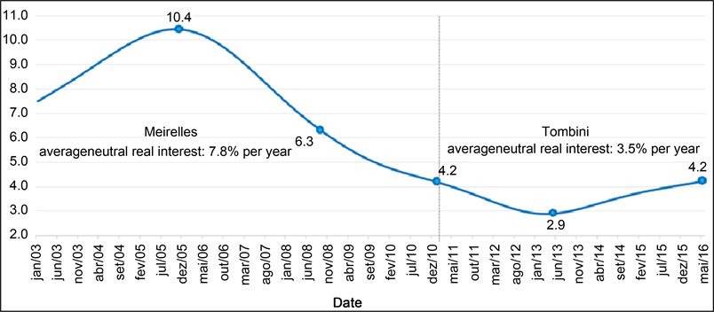
Chart 1. Monthly estimates for the neutral real interest rate (%): HP filter. Source: elaborated by the authors.

Chart 2. Annual estimates for the neutral real interest rate (%): HP filter. Source: elaborated by the authors.

Furthermore, by calculating the average for the ex-post and neutral interest rates, the average of the neutral rate in the period is 7.0, while the average of the ex-post rate is 8.7. The lower average of the neutral interest rate compared to the ex-post rate indicates that the CB can more easily foresee the neutral real interest rate, which allows it to guide monetary policy with greater assertiveness when monitoring inflation projections, evidencing the usefulness of the neutral real interest rate in terms of constructing a reaction function for monetary policy.

As for the interest rate gap and monthly inflation, although the interest rate gap is almost always positive throughout the period analyzed (its average is 1.2 percentage points), the inflation rate does not show a tendency to fall in the

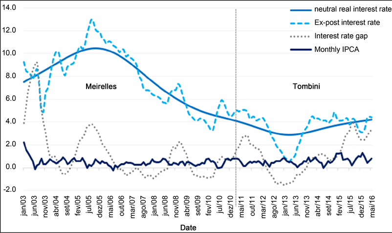
Chart 3. Interest rate gap, ex-post interest, neutral real interest (HP filter), and monthly IPCA (%). Source: elaborated by the authors.

analysis horizon, which contradicts the economic theory, according to which a positive interest rate gap would lead to decreasing inflation. It should be noted that, in any case, this would not happen contemporaneously given the lagged effects of monetary policy.

Despite the simplicity that the implementation of the HP filter provides in estimating the neutral real interest rate, it should be noted, however, that this method has significant limitations, especially the so-called end-point bias, in which the long end of the trend obtained by the HP filter is strongly affected by the final data of the series, so that the trend component of the estimate may be affected by the business cycle.

4.2. Estimates Generated by the SVAR Model

Following Brzoza-Brzezina (2003) , the monthly estimates of the neutral real interest rate obtained by applying the SVAR model were obtained using the series of the ex-ante domestic basic interest rate (Selic rate deflated by the expectation of inflation measured by IPCA 12 months ahead) and the first difference of the accumulated inflation in 12 months measured by IPCA. These variables were used in these formats due to the results of the stationarity tests performed (in this case, the ADF test was implemented). The monthly time series of the neutral real interest rate obtained with the implementation of the SVAR is shown in Chart 4.

Chart 4. Monthly estimates for the neutral real interest rate (%): SVAR. Source: elaborated by the authors.

By visually inspecting the charts, one can note that such estimates are considerably more volatile than those obtained by implementing the HP filter, which can be attributed to the fact that in SVAR, the average real interest is added to the neutral interest to obtain the final estimate. This explains the single average for the neutral interest rate in both terms.

In turn, Chart 5 presents, in addition to the estimate for the neutral real interest rate, the ex-post real interest rate, the interest rate gap, and monthly inflation measured by the IPCA.

In this case, we observed an interest rate gap even larger than the one verified in the estimation implementing the HP filter. Moreover, by calculating the variance for the ex-post and neutral rates, the variance of the neutral rate in the period is 0.4, while the variance of the ex-post rate is 8.7, suggesting, as in the previous estimate, that the CB can more easily predict the neutral rate, which allows it to guide monetary policy with greater assertiveness.

With respect to the interest rate gap and monthly inflation, a primarily negative gap is verified over the analyzed period (its average is −0.6 percentage points). In turn, the inflation rate shows no downward trend over the horizon of analysis, remaining relatively stable, a result that differs significantly from that found using the HP filter. In this case, in economic theory, a negative interest rate gap would lead to rising inflation.

4.3. Comparison between the Methods Employed, Combined Estimation, and Considerations about the Monetary Policy

Comparing the two implemented methods, we highlight that each of the models

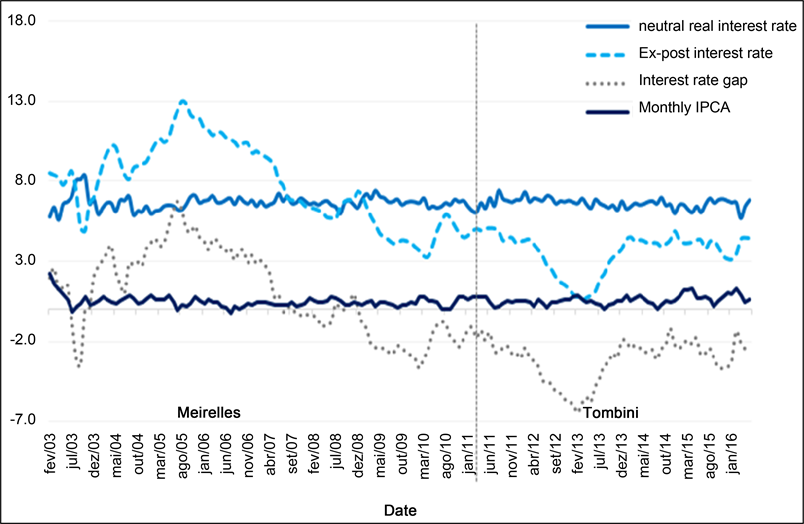
Chart 5. Interest rate gap, ex-post interest, neutral real interest rate (SVAR model), and monthly IPCA (%). Source: elaborated by the authors.

Chart 6. Estimates for the neutral real interest rate (%): HP, SVAR, and “combined rate”. Source: elaborated by the authors.

used has a profile and captures different information, making them complementary. Because of this, the “combined rate” returns a smoother estimate, reducing the uncertainty inherent to estimating a latent variable such as the neutral interest rate, which is the main contribution of this paper compared to other available studies. It is also worth mentioning the fact that, in the HP filter, there is a significant interest rate gap at several moments, a movement that is quite different in the SVAR, in which the gap is considerably smaller, given that, in the first method, the bias component of the neutral interest rate estimate tends to be affected by the business cycle.

Illustrated in Chart 6, one can see that the trajectory of the combined rate does not allow one to affirm that the neutral interest rate presented a relevant reduction during Tombini’s mandate. This is due to the relative stability of the neutral rate estimate resulting from implementing the SVAR model, suggesting that his management was marked by discretion in the conduct of monetary policy.

5. Conclusion

From a modern point of view, the neutral rate, as the name implies, is one that denotes the “neutral” action of a Central Bank given that, by pursuing it, the monetary authority ensures price stability and, at the same time, does not exert any influence on the product. More specifically, the neutral interest rate represents the interest rate in force at the moment when monetary policy is neither expansionary (aimed at stimulating activity) nor contractionary (practiced discouraging the economy). In this context, it can be said that the neutral interest rate serves as a reference to guide (expansionary or contractionary) the Central Bank’s monetary policy, so that in an inflation-targeting regime, knowing this variable enables the monetary authority to determine the path of nominal interest rates, its monetary policy instrument, to ultimately reach the target price level, which in turn minimizes product level volatility.

It should be noted that the neutral interest rate does not represent an explicitly observable measure, so that, to know it, it is necessary to estimate it. Indeed, the neutral interest rate estimates, even for countries with numbers much lower than in Brazil, have a wide confidence interval. In view of this, one must recognize the existence of risks in following a strategy of setting nominal interest rates based on a measure as uncertain as the neutral interest rate, which tends to produce noise in the conduct of monetary policy, consequently causing economic instability.

Given these circumstances, this paper aimed to estimate the structural interest rate of the Brazilian economy from January 2003 to May 2016, a variable that, although not explicitly observable, is pivotal in discussions of economic policy. In fact, knowing the neutral interest rate and understanding its temporal dynamics is pivotal for defining and analyzing monetary policy decisions.

In terms of structure, after a brief literature review and presenting the methods used in this paper, the estimations were performed, which were operationalized through three different methods: the Hodrick-Prescott filter and a structural VAR model. After the estimations were performed, they were all combined, resulting in a single Brazilian neutral interest rate estimate. It is noteworthy that the strategy of combining both implemented methods was adopted because each of them has a profile and provides different information, making them complementary, in addition to returning a smoother estimate and reducing the uncertainty inherent in estimating a latent variable such as the neutral interest rate, thereby being the main contribution of this study compared to other works.

The sample used in the estimations began in January 2003, and ended in May 2016, a period with a constant monetary policy in qualitative terms, since, in this interregnum, there was no change in the monetary policy regime, with the inflation-targeting regime in force. Another justification for the choice is that this time frame has numerous monthly observations and contains all the necessary data to enable the estimations.

Lastly, the main results of this study revealed that it is not possible to affirm that the neutral interest rate presented a relevant reduction during the period Alexandre Tombini was in charge of the Central Bank, suggesting that his management was marked by discretion in the conduct of monetary policy.

NOTES

¹It is important to note that, despite the existence of two solutions for $s_{1,1}\left(0\right)$ and $s_{2,1}\left(0\right)$ , the solution for the neutral real interest rate is unique.

Conflicts of Interest

The authors declare no conflicts of interest regarding the publication of this paper.

References

[1]	Amato, J. (2005). The Role of the Natural Rate of Interest in Monetary Policy. Bank of International Settlements, BIS Working Paper 171. https://doi.org/10.2139/ssrn.699221
[2]	Archibald, J., & Hunter, L. (2001). What Is the Neutral Real Interest Rate and How Can We Use It. Reserve Bank of New Zealand Bulletin, 63, 15-28.
[3]	Arida, P., Bacha, E. L., & Lara-Resende, A. (2004). Credit, Interest and Jurisdicional Uncertainty: Conjectures on the Case of Brazil. Instituto de Estudos de Política Econômica, Casa das Garças, Rio de Janeiro.
[4]	Banco Central do Brasil (2017). Sistema Gerenciador de Séries Temporais. https://www3.bcb.gov.br/sgspub
[5]	Barbosa, F. H. (2006). The Contagion Effect of Public Debt on Monetary Policy: The Brazilian Experience. Revista de Economia Política, 26, 231-238. https://doi.org/10.1590/S0101-31572006000200004
[6]	Barbosa, F. H., Camêlo, F. D., & João, I. C. (2016). A Taxa de Juros Natural e a Regra de Taylor no Brasil: 2003-2015. RevistaBrasileira de Economia, 70, 399-417. https://doi.org/10.5935/0034-7140.20160021
[7]	Barcellos Neto, P. C. F., & Portugal, M. S. (2009). The Natural Rate of Interest in Brazil between 1999 and 2005. Revista Brasileira de Economia, 63, 103-118. https://doi.org/10.1590/S0034-71402009000200003
[8]	Blanchard, O., & Quah, D. (1989). The Dynamics Effects of Aggregate Demand and Supply Disturbances. American Economic Review, 79, 655-673. https://doi.org/10.3386/w2737
[9]	Blinder, A. (1998). Central Banking in Theory and Practice. The MIT Press.
[10]	Borges, B. L. (2017). Como reduzir o juroestrutural no Brasil: O caminho das pedras. Blog do Instituto Brasileiro de Economia (IBRE). http://blogdoibre.fgv.br/posts/como-reduzir-o-juro-estrutural-no-brasil-o-caminho-das-pedras
[11]	Borges, B. L., & Silva, M. B. S. (2006). Estimando a taxa de juros natural para o Brasil: Uma aplicação da metodologia VAR estrutural. Estudos Econômicos, São Paulo, 36, 87-114. https://doi.org/10.1590/S0101-41612006000100004
[12]	Bresser Pereira, L. C., & Nakano, Y. (2002). Aarmadilha dos juros. Folha de São Paulo, 10 de fevereiro de.
[13]	Brzoza-Brzezina, M. (2003). Estimating the Natural Rate of Interest: A SVAR Approach. National Bank of Poland Working Paper.
[14]	Favero, C. A., & Giavazzi, F. (2002). Why Ate Brazil’s Interest Rates to High? Working Paper No. 224, IGIER-Università Bocconi.
[15]	Fuhrer, J. C., & Moore, G. R. (1993). Forward-Looking Behavior of Long-Term Interest Rates. Working Paper in Applied Economic Theory, Federal Reserve Bank of San Francisco.
[16]	Goldfajn, I., & Bicalho, A. (2011). A longa travessia para a normalidade: Osjurosreais no Brasil. https://www.itau.com.br/itaubba-pt/analises-economicas/publicacoes/textos- para-discussao/a-longa-travessia-para-a-normalidade-os-juros-reais-no-brasil
[17]	Gotlieb, J. W. F. (2013). Estimativas e Determinantes da Taxa de Juros Real Neutra do Brasil. Dissertação de Mestrado, Departamento de Economia, Pontifícia Universidade Católica do Rio Janeiro.
[18]	Hodrick, R., & Prescott, E. (1997). Postwar U.S. Business Cycles: An Empirical Investigation. Journal of Money, Credit, and Banking, 29, 1-16. https://doi.org/10.2307/2953682
[19]	Holston, K., Laubach, T., & Williams, J. C. (August, 2016). Measuring the Natural Rate of Interest: International Trends and Determinants. Board of Governors of the Federal Reserve System.
[20]	Laubach, T., & Williams, J. C. (November, 2003). Measuring the Natural Rate of Interest. Board of Governors of the Federal Reserve System.
[21]	Mésonnier, J. S., & Renne, J. P. (2007). A Time-Varying “Natural” Rate of Interest for the Euro Area. European Economic Review, 51, 1768-1784. https://doi.org/10.1016/j.euroecorev.2006.11.006
[22]	Miranda, P. C., & Muinhos, M. K. (2003). A taxa de juros de equilíbrio: Uma abordagem múltipla. Trabalho para discussão n. 66, Banco Central do Brasil.
[23]	Muinhos, M. K., & Nakane, M. (2006). Comparingequilibrium Real Interest Rates: Different Approaches to Measure Brazilian Rates. Working Paper No. 101, Banco Central do Brasil, Março. https://www.bcb.gov.br/pec/wps/ingl/wps101.pdf
[24]	Orphanides, A., & Williams, J. (April, 2006). Inflation Targeting under Imperfect Knowledge. Federal Reserve Bank of San Francisco Working Paper Series, No. 14. https://doi.org/10.24148/wp2006-14
[25]	Perrelli, R., & Roache, S. K. (2014). Time-Varying Neutral Interest Rate: The Case of Brazil. Working Paper No. 14/84, International Monetary Fund. https://www.imf.org/external/pubs/cat/longres.aspx?sk=41552.0 https://doi.org/10.5089/9781484385210.001
[26]	Ribeiro, A., & Teles, V. K. (2013). Taxa natural de juros para oBrasil. Economia, 14, 733-750. http://www.anpec.org.br/revista/aprovados/Natural.pdf
[27]	Schwartsman, A. (2011). Sobre Jabutis e Jabuticabas. Jornal Valor Econômico.
[28]	Wicksell, K. (1898). Interest and Prices (Translated by R. F. Kahn in 1936). Sentry Press.
[29]	Woodford, M. (2003). Interest and Prices: Foundations of a Theory of Monetary Policy. Princeton University Press. https://doi.org/10.1515/9781400830169