Potential Power of the Pyramidal Structure VII: Effects of Pyramid Power and Bio-Entanglement on the Circadian Rhythm of Biosensors ()
1. INTRODUCTION
Vegetables and fruits are known to have long-lasting biological reactions even after harvesting. And when the plants are subjected to some stimulation or injury after harvest, they may release various types of volatile components. Plants use these volatile components for communication with other plants, defense against foreign enemies, and immune actions [1 - 10].
As biosensors we have been using cucumber sections, Cucumis sativus, which release volatile components. By measuring and analyzing the concentrations of gas emitted from the biosensors, we have revealed unexplained phenomena that could not have previously been captured by regular electrical instruments [11 , 12].
Unexplained functions, a pyramid power which a pyramidal structure (PS) is said to have are of great scientific interest. Since October 2007, we have been conducting rigorous scientific experiments using the biosensors on a pyramid in which a test subject can enter and meditate in order to elucidate the unexplained power of the pyramidal structure, the pyramid power (Figure 1). In parallel, we are also studying the characteristics of the biosensors. We have demonstrated the existence of the pyramid power and have revealed its characteristics. Our studies also revealed the existence of a circadian rhythm in which the gas concentrations emitted from the biosensors varies with the seasons. As a result of our research to date, we have published 10 original papers demonstrating the pyramid effect [13 - 22], 3 original papers characterizing cucumbers used as the biosensors [23 - 25], 3 comprehensive reports [26 - 28], and 1 book [29]. Analysis of the pyramid effect on the biosensors revealed the existence of a phenomenon similar to quantum entanglement between cucumber sections due to pyramid power, which we named Bio-Entanglement [20 - 22].
In a previous paper, we reported that the circadian rhythm of gas concentrations emitted from biosensors changes seasonally, i.e., the circadian cycle is 8 hours in winter, 6 hours in spring, 24 hours in summer, and a mixed cycle of 12 and 24 hours in autumn [25]. In the experiment, eight biosensors GE1, GE2, GE3, GE4, GC1, GC2, GC3, GC4 were placed as shown in Figure 1(c). We found that all eight gas concentrations had different circadian rhythms at different seasons: GE1 and GE2 were affected by the pyramid power, GC1 and GC2 were affected by the Bio-Entanglement, and GE3, GE4, GC3 and GC4 of the control placed at the calibration control point, oscillated in the same way. Thus, at the time the paper was published [25], we had found that the pyramid power and the Bio-Entanglement had no effect on the number of cycles of the circadian rhythm of gas concentration.
The purpose of this paper is to analyze whether or not there are any effects on anything other than the number of cycles. Specifically, the phase and amplitude of the periodic approximation curve representing the circadian rhythm of the gas concentration emitted from the biosensors and the correlation coefficient between the gas concentration and its periodic approximation curve are studied in detail, and the influences of the pyramid power and the Bio-Entanglement on the phase, amplitude and correlation coefficient are analyzed.
2. PREPARATION, INSTALLATION AND STORAGE OF THE BIOSENSORS, AND GAS CONCENTRATION MEASUREMENT OF THE BIOSENSORS
In one set of pyramid power detection experiments, eight uniform biosensors GE1, GE2, GE3, GE4, GC1, GC2, GC3, GC4 were prepared from four commercial edible cucumbers (Figure 1(a) and Figure 1(b)). To prepare eight uniform biosensors, each Petri dish contains four cucumber sections, one from each of the four cucumbers. In pairs 1 to 4 shown in Figure 1(b), the surfaces of the cucumber sections for each pair are identical cut surfaces. However, only the direction of the cut surface is different. That is, GE1, GE2, GE3, and GE4 are experimental samples and the direction of the cut surface is the same as the growth axis, while GC1, GC2, GC3, and GC4 are control samples and the direction of the cut surface is opposite to the growth axis (Figure 1(a), lower panel). GE1, GE2, GE3, GE4, GC1, GC2, GC3, and GC4 represent the Petri dishes of the eight biosensors, as well as the gas concentrations (ppm) released from the biosensors in each Petri dish.
![]()
Figure 1. Preparation and placement of biosensors. (a) The process of preparing four pairs of biosensors by cutting 32 cucumber sections of 1 cm width from four cucumbers. (b) Eight uniform biosensors from pairs 1 to 4 were prepared and placed at the PS apex and calibration control point. (c) Two biosensors were stacked on top of each other and placed at the PS apex and the calibration control point 8 m away.
The reason for using eight uniform biosensors in one set of experiments was to utilize the Simultaneous Calibration Technique (SCAT) devised at the International Research Institute (IRI) in experiments to detect healing and pyramid power effects [30]. SCAT is a sensing method that reveals spatial characteristics using biosensors, which are considered environmentally responsive, highly sensitive sensors. This method eliminates data bias due to individual differences in cucumbers and changes in environmental conditions. This made it possible to detect weak effects affecting the cucumber gas production reaction that would otherwise be buried as noise. And we have been able to detect human healing capacity [11 , 12] and pyramid power [13 - 29], which were difficult to detect by regular electrical instruments.
In the experiment, GE1 and GE2 were placed at the PS apex in two layers. GC1, GC2, GE3, GE4, GC3, and GC4 were placed at the calibration control point 8 m away from the PS apex in two layers (Figure 1(c)). The biosensors GE3, GE4, GC3, and GC4 of pairs 3 and 4 were under the same environment from preparation to installation at the calibration control point and storage after installation. Therefore, the four biosensors were assumed to have the same biological response to produce the gas and could serve as controls. The biosensors were placed at the PS apex and the calibration control point simultaneously for 30 min, then the Petri dish lids were removed, and the dishes with the biosensors were placed in a sealed polypropylene container with a volume of 2.2 liters, and stored in a temperature-controlled (22 - 24 degrees Celsius) room with no direct sunlight for 24 h - 48 h. During storage, the gas concentration in the sealed container has been found to reach a maximum in about 12 hours and then remain in equilibrium [31]. Gas concentration was measured by aspirating 300 ml of gas in a sealed container using a gas detector (GV-100: GASTEC, Japan) and a gas detector tube (141 L: GASTEC).
It has been reported that there are 16 main gas components released from cucumber sections, and we understand that we are measuring the concentration of 2-hexanol among them [32 , 33]. The reason for this is that the gas detector tube 141 L is originally intended for ethyl acetate detection, but 2-hexanol is detectable. However, when identifying the absolute value of the 2-hexanol gas concentration, it was necessary to multiply the detector tube reading (ppm) by three from the conversion factor. The 16 mixtures of gases released from cucumbers include isomers of 2-hexanol and other compounds. Therefore, to obtain an accurate value for the gas concentration, the composition ratio of the 2-hexanol isomer and the conversion factor are needed, but these are not known at this time. However, the purpose of this paper is not to determine the absolute value of gas concentrations emitted from cucumber sections, but to determine the effects of the pyramid power and the Bio-Entanglement on the periodic approximation curve representing the circadian rhythm of gas concentrations. Therefore, we used the detector tube reading (ppm) as the gas concentration in our analysis.
3. PERIODIC APPROXIMATION CURVE OF GAS CONCENTRATION
To clarify the circadian rhythm of gas concentration, we first obtained a periodic approximation curve of gas concentration that repeats the same phase every 24 hours. The correlation between gas concentration and the periodic approximation curve was then analyzed, and the correlation coefficient and its significance were examined to determine if a circadian rhythm existed in gas concentration.
We used Equation (1) as the periodic approximation curve.
(1)
Here, a, b, and c are constants, and π is the circumference ratio. The variable x represents the time, and it is a value corresponding to the time from 0:00 to 24:00 with a numerical value from 0 to 1. If the post-harvest cucumbers maintained a circadian rhythm, the gas concentrations released by the biological response were also assumed to follow a circadian rhythm that was in phase every 24 hours. N is the number of cycles per 24 hours and here we consider N to be an integer from 1 to 24. Equation (1) therefore represents the period approximation curve with one period of 24 hours for N = 1 and one period of 1 hour for N = 24. We determined the periodic approximation curves for each of the eight gas concentrations GE1, GE2, GE3, GE4, GC1, GC2, GC3, and GC4 for N ranging from 1 to 24 and determined the constants a, b, and c. The correlation coefficient between the gas concentration and the periodic approximation curve was then calculated. If the correlation coefficient was significant, we considered the period of the periodic approximation curve to be the period of the circadian rhythm of the gas concentration.
4. CIRCADIAN RHYTHM OF GAS CONCENTRATION
The data used in this paper to analyze the circadian rhythm of gas concentrations were the same data used in the six-paper series “Potential Power of the Pyramidal Structures I-VI” [17 - 22] and in the previously published paper [25]. All data (n = 468) were analyzed separately for each of the four seasons: WTR (n = 84), SPR (n = 108), SMR (n = 144), and AUT (n = 132) (Table 1). In this paper, we analyzed the circadian rhythm of the gas concentration of each of the eight biosensors, always recognizing the differences between how the pyramid power affected biosensors GE1 and GE2, the Bio-Entanglement affected biosensors GC1 and GC2, and the control biosensors GE3, GE4, GC3, and GC4, as well as between the two stacked lower and upper layers of biosensors in the experiment.
![]()
Table 1. Classification of the four seasons and their duration, as well as the number of data for each season.
Figure 2 shows the correlation coefficients between the eight gas concentrations GE1, GE2, GE3, GE4, GC1, GC2, GC3, GC4 and the periodic approximation curve. The vertical axis is the correlation coefficient. The horizontal axis is the number of cycles N of the periodic approximation curve per 24 hours, an integer from 1 to 24. The four dashed lines in the figure represent the significance of the correlation coefficients, which vary with the number of data. The red dashed line represents the significance of p = 10−5, the green dashed line p = 10−4, the blue dashed line p = 10−3, and the black dashed line p = 10−2. Figure 2(a) shows the results for winter (WTR), Figure 2(b) for spring (SPR), Figure 2(c) for summer (SMR), and Figure 2(d) for autumn (AUT). Based on the results in Figure 2, we determined that the circadian rhythm of the gas concentrations emitted from the biosensors has one cycle of 8 hours (N = 3) for WTR, 6 hours (N = 4) for SPR, 24 hours (N = 1) for SMR, and a mixture of 24 hours (N = 1) and 12 hours (N = 2) for AUT [25].
Figure 3 and Figure 4 show the periodic approximation curves representing the circadian rhythms of the eight gas concentrations identified in Figure 2. Vertical axis is gas concentration. Horizontal axis is time from 0:00 to 24:00 (0:00). The red solid, red dashed, black solid and black dashed lines represent GE1, GE2, GE3 and GE4, respectively, while the blue solid, blue dashed, gray solid and gray dashed lines represent GC1, GC2, GC3 and GC4, respectively. Figure 3(a) shows the results for WTR (8-hour period with N = 3), Figure 3(b) for SPR (6-hour period with N = 4), Figure 3(c) for SMR (24-hour period with N = 1), Figure 4(a) for AUT (24-hour period with N = 1), Figure 4(b) for AUT (12-hour period with N = 2) and Figure 4(c) for AUT (a combination of N = 1 and N = 2). Comparing SMR (Figure 3(c)) and AUT (Figure 4(a)), which has a circadian rhythm with one cycle of 24 hours, we found that the peak position of the periodic approximation curve deviated by about 4 hours, indicating that the phase of the circadian rhythm shifted significantly depending on the season even though the period was the same.
Figure 3 and Figure 4 show that the phase and amplitude of the periodic approximation curves representing the circadian rhythms of eight different gas concentrations in each season were slightly different. Whether this difference was due to experimental error or the result of the influences of the pyramid power and the Bio-Entanglement was analyzed next.
5. EFFECTS OF THE PYRAMID POWER AND THE BIO-ENTANGLEMENT ON CIRCADIAN RHYTHMS OF GAS CONCENTRATION
5.1. Effects of Pyramid Power and Bio-Entanglement on Phase
Table 2 shows the peak times of the periodic approximation curves representing the circadian rhythm of gas concentrations for each season. Here, E1, E2, E3, E4, C1, C2, C3 and C4 represent the peak times of the periodic approximation curves for the circadian rhythm of gas concentrations GE1, GE2, GE3, GE4, GC1, GC2, GC3 and GC4. If there is more than one peak, we chose the time of the peak that appeared closest to time 0:00. In each seasonal column, the left side is the peak time, and the right side is the value of the peak time when the time 0:00-24:00 corresponds to the value 0 - 1.
![]()
Figure 2. The correlation coefficients between the eight gas concentrations GE1, GE2, GE3, GE4, GC1, GC2, GC3, GC4 and the periodic approximation curve. The vertical axis is the correlation coefficient. The horizontal axis is the number of cycles N of the periodic approximation curve per 24 hours, an integer from 1 to 24. The four dashed lines in the figure represent the significance of the correlation coefficients, which vary with the number of data. The red dashed line represents the significance of p = 10−5, the green dashed line p = 10−4, the blue dashed line p = 10−3, and the black dashed line p = 10−2. (a) WTR, (b) SPR, (c) SMR, (d) AUT.
![]()
Figure 3. The periodic approximation curves representing the circadian rhythms of the eight gas concentrations identified in Figure 2. Vertical axis is gas concentration. Horizontal axis is time from 0:00 to 24:00 (0:00). The red solid, red dashed, black solid and black dashed lines represent GE1, GE2, GE3 and GE4, respectively, while the blue solid, blue dashed, gray solid and gray dashed lines represent GC1, GC2, GC3 and GC4, respectively. (a) WTR; N = 3, (b) SPR; N = 4, (c) SMR; N = 1.
![]()
Table 2. Peak times of the periodic approximation curves representing the circadian rhythm of gas concentrations. E1, E2, E3, E4, C1, C2, C3 and C4 represent the peak times of the periodic approximation curves for the circadian rhythm of gas concentrations GE1, GE2, GE3, GE4, GC1, GC2, GC3 and GC4. If there are multiple peaks in the periodic approximation curve, the peak that appears at the earliest time from 0:00 is shown. In each season, the left side is the peak time, and the right side is the value when the time 0:00-24:00 corresponds to the value 0 - 1.
![]()
Figure 4. The periodic approximation curves representing the circadian rhythms of the eight gas concentrations identified in Figure 2. Vertical axis is gas concentration. Horizontal axis is time from 0:00 to 24:00 (0:00). The red solid, red dashed, black solid and black dashed lines represent GE1, GE2, GE3 and GE4, respectively, while the blue solid, blue dashed, gray solid and gray dashed lines represent GC1, GC2, GC3 and GC4, respectively. (a) AUT; N = 1, (b) AUT; N = 2, (c) AUT; N = 1 & 2.
Table 3 is a matrix table of correlation coefficients obtained by the analysis of 1) - 3) shown below. 1) Twenty-eight combinations of peak times E1, E2, E3, E4, C1, C2, C3, and C4 of the periodic approximation curves representing the eight circadian rhythms shown in Table 2 were obtained, for example, (E1, E2), (E1, E3), (E1, E4), etc. 2) With the 28 combinations, the difference was calculated for each season to obtain the seasonal phase difference; for example, WTR (E1 − E2), SPR (E1 − E2), SMR (E1 − E2), AUT-1 (E1 − E2), AUT-2 (E1 − E2), etc. 3) Correlation coefficients were calculated between seasonal phase differences; for example, correlation coefficients were calculated between (WTR (E1 − E2), SPR (E1 − E2), SMR (E1 − E2), AUT-1 (E1 − E2), AUT-2 (E1 – E2)) and (WTR (E1 − E3), SPR (E1 − E3), SMR (E1 − E3), AUT-1 (E1 − E3), AUT-2 (E1 − E3)). The number of phase difference data was n = 5 (WTR N = 3, SPR N = 4, SMR N = 1, AUT N = 1, AUT N = 2).
The first column and first row of Table 3 show the difference between the 28 different peak times. In the colored areas in Table 3, red indicates areas that suggest the effect of the pyramid power, blue indicates areas that suggest the effect of the Bio-Entanglement, green indicates the difference between the lower and upper layers, and orange indicates the difference between pairs. In Table 3, the areas ①through ⑩, represented in yellow, are those where the correlation coefficient was greater than 0.959 and the correlation coefficient met the 1% significance level. We chose the yellow part because, when the number of data was n = 5, the significance of the correlation coefficient was calculated and found to be 1% significant if the correlation coefficient was greater than 0.959.
Table 3. Correlation coefficients between phase differences in the periodic approximation curves representing the circadian rhythm of gas concentration. Red indicates areas that suggest the effect of the pyramid power, blue indicates areas that suggest the effect of the Bio-Entanglement, green indicates the difference between the lower and upper layers, and orange indicates the difference between pairs. The areas ①through ⑩, represented in yellow, are those where the correlation coefficient was greater than 0.959.
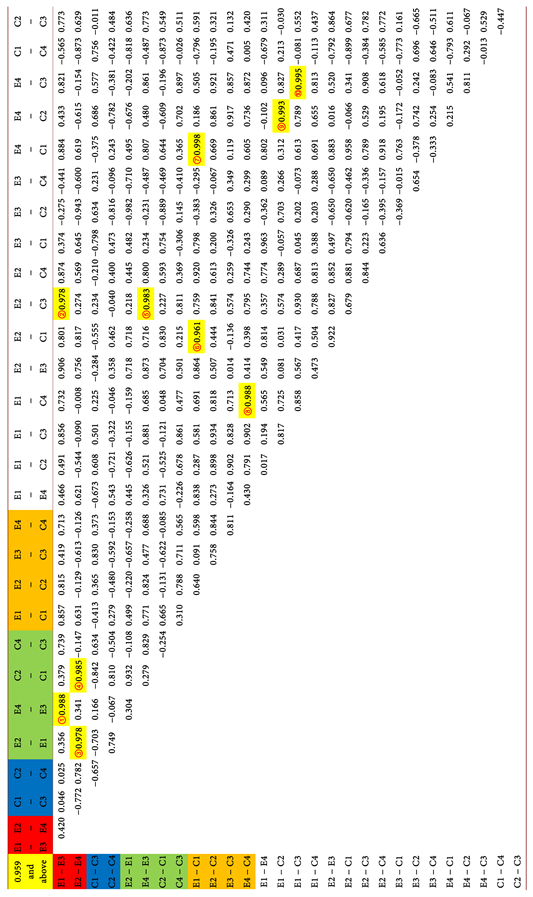
Figure 5 shows the results of examining the areas ①through ⑩highlighted in yellow in Table 3. Correlation coefficients from ①to ⑩were 1% significant. We therefore assumed that the difference between the phase difference and the phase difference was a constant, and we formulated the equations for ①through ⑩, respectively; that is, the ten equations ①E1 − E3 = E4 − E3 + a, ②E1 − E3 = E2 − C3 + b, …, ⑩E1 − C3 = E4 − C3 + j. Here, a to j are constants. The 10 equations were not all independent, and after rearranging them, equations (i) through (v) in Figure 5 remained (actually, equation (iii) can be derived from (iv) and (v), but we decided to leave it here).
Figures 6(a)-(j) show the seasonal changes in phase differences for the columns and rows corresponding to ①-⑩in Table 3. The vertical axis represents time, with a value of 1 corresponding to 24 hours. The horizontal axis is the season and the number of cycles of its circadian rhythm, N. The correlation coefficients between phase differences from ①to ⑩were greater than 0.959, indicating that the seasonal changes in phase differences were almost qualitatively the same. The values of a - j in Figures 6(a)-(j) were the average of the seasonal phase difference minus the phase difference, e.g., the value of a was the average of the seasonal phase difference (E1 − E3) minus the phase difference (E4 − E3) in Figure 6(a). When calculating the values of a - j, we always subtracted the columns (circles in Figure 6) from the rows (triangles in Figure 6) corresponding to ①through ⑩in Table 3. Table 4 shows the values of a - j calculated from Figures 6(a)-(j).
We next considered equations (i) - (v) in Figure 5. From equation (iv) and Table 4, E2 − E1 = −f = −0.0087. (E2 − E1) was the average of the circadian rhythm phase difference in gas concentrations between GE2, the upper layer and GE1, the lower layer which is affected by the pyramid power. Since the mean of the phase difference was −0.0087, the phase of the circadian rhythm of GE2 was shifted to the left by 12.5 min relative to GE1. From equation (v) and Table 4, C2 − C1 = a − d − f = −0.0094. (C2 − C1) was the average of the circadian rhythm phase difference in gas concentrations between GC2, the upper layer and GC1, the lower layer which is affected by the Bio-Entanglement. Since the mean of the phase difference was −0.0094, the phase of the circadian rhythm of GC2 was shifted to the left by 13.5 min relative to GC1. Next, by adding equations (i) and (iv), we obtained E2 − E4 = a − f = −0.0298. Since GE2 and GE4 were both in the upper layer, GE2 being affected by the pyramid power and GE4 being the control, (E2 − E4) represented the phase shift of the circadian rhythm of GE2 due to the pyramid power. With a phase difference of −0.0298, we found that the pyramid power shifted the phase of GE2 43 min to the left.
![]()
Figure 5. Consideration of correlation coefficients ①through ⑩that are greater than 0.959 in Table 3.
![]()
Table 4. Values of constants a - j calculated from the graphs in Figures 6(a)-(j).
![]()
Figure 6. Graphical representation of ①through ⑩where the correlation coefficient was 0.959 or higher in Table 3. The value of (a) - (j) in the figure is the average of the difference between the two graphs in (a) - (j) for each season.
5.2. Effects of Pyramid Power and Bio-Entanglement on Amplitude
Figure 7 shows the ratio of the amplitudes of the periodic approximation curves representing the circadian rhythms of the gas concentrations GE1, GE2, GE3, GE4, GC1, GC2, GC3 and GC4. The amplitudes of the gas concentrations GE1, GE2, GE3, GE4, GC1, GC2, GC3 and GC4, are e1, e2, e3, e4, c1, c2, c3, and c4, respectively. The horizontal axis is the season and the number of cycles of its circadian rhythm, N.
Figure 7(a) shows the amplitude ratios e2/e1, e4/e3, c2/c1, and c4/c3. Here, the denominators e1, e3, c1, and c3 are the amplitudes of the gas concentrations of the biosensors in the lower layer, and the numerators e2, e4, c2, and c4 are the amplitudes of the gas concentrations of the biosensors in the upper layer. The results showed a difference between the lower and upper layers with respect to the amplitude of the circadian rhythm. The ratio between controls, e4/e3 (black squares) and c4/c3 (gray squares), always had a ratio value greater than 1, indicating that the amplitude of the upper layer was greater than that of the lower layer. The value of the ratio was particularly large in SPR. From this we understood that in the control, the gas release activity was greater in the upper GE4, GC4 than in the lower GE3, GC3. Possible reasons for this are that during the experiment, the upper layer was exposed to more lighting than the lower layer, and the temperature might be higher in the upper layer than in the lower layer. Furthermore, we considered why the ratio was greater in the SPR. The reason is that the biological response to gas release was more active in the SPR than in other seasons. On the other hand, the ratio of the amplitudes of the biosensors GE1 and GE2 affected by the pyramid power, e2/e1 (red squares), had values less than 1 from WTR to SMR, and the activity of gas emission in the upper layer GE2 appeared to be suppressed compared to that in the lower layer GE1. The ratio c2/c1 (blue squares) of the amplitudes of the biosensors GC1 and GC2 affected by the Bio-Entanglement changed qualitatively the same as e2/e1 affected by the pyramid power. In the WTR, however, the ratio values were greater than 1, consistent with the control ratios e4/e3 and c4/c3.
Figure 7(b) shows e1/e3 and e2/e4, the ratios of e1 and e2 affected by the pyramid power to e3 and e4 in the control, and c1/c3 and c2/c4, the ratios of c1 and c2 affected by the Bio-Entanglement to c3 and c4
![]()
Figure 7. The ratio of the amplitudes of the periodic approximation curves representing the circadian rhythms of the gas concentrations GE1, GE2, GE3, GE4, GC1, GC2, GC3 and GC4. The amplitudes of the gas concentrations GE1, GE2, GE3, GE4, GC1, GC2, GC3 and GC4 are e1, e2, e3, e4, c1, c2, c3, and c4, respectively. The horizontal axis is the season and the number of cycles of its circadian rhythm, N. (a) The amplitude ratios e2/e1, e4/e3, c2/c1, and c4/c3. (b) The amplitude ratios e1/e3, e2/e4, c1/c3, and c2/c4.
in the control. Here, the ratio between the lower layers is indicated by circles and the ratio between the upper layers is indicated by triangles. Thus, Figure 7(b) shows how the effects of the pyramid power and the Bio-Entanglement affected the amplitude of the circadian rhythm of gas concentrations. For the pyramid power effect, the ratio e1/e3 between the lower layers was always larger than 1 in value. It was especially large in SPR. The ratio e2/e4 between the upper layers had a value less than 1 from WTR to SMR and a value greater than 1 in AUT. For the Bio-Entanglement effect, the ratio c1/c3 between the lower layers was qualitatively almost equal to the effect of the pyramid power. The ratio of c2/c4 between the upper layers was also qualitatively equal to the effect of the pyramid power, with values less than 1 from WTR to SMR. These suggested that the effects of the pyramid power and the Bio-Entanglement on the amplitude of the circadian rhythm of gas concentration were qualitatively the same and that the effect sizes were proportional.
5.3. Effects of Pyramid Power and Bio-Entanglement on Correlation Coefficient
Figure 8 shows the seasonal variation of the correlation coefficient between gas concentration and the periodic approximation curve representing the circadian rhythm of gas concentration shown in Figure 3 and Figure 4. The vertical axis is the correlation coefficient. The horizontal axis is the season and the number of cycles of its circadian rhythm, N. In particular, AUT has three cases, N = 1, N = 2, and N = 1 & 2. Here, the correlation coefficients between the gas concentrations GE1, GE2, GE3, GE4, GC1, GC2, GC3, GC4 and the periodic approximation curve representing the circadian rhythm of the gas concentrations are expressed as gE1, gE2, gE3, gE4, gC1, gC2, gC3, gC4.
![]()
Figure 8. The seasonal variation of the correlation coefficient between gas concentration and the periodic approximation curve representing the circadian rhythm of gas concentration shown in Figure 3 and Figure 4. The vertical axis is the correlation coefficient. The horizontal axis is the season and the number of cycles of its circadian rhythm, N. (a) The correlation coefficients gE1 and gE2 affected by the pyramid power. (b) The correlation coefficients gC1 and gC2 affected by the Bio-Entanglement. (c) and (d) The correlation coefficients gE3, gE4, gC3 and gC4 for the controls.
Figure 8(a) shows the correlation coefficients gE1 and gE2 affected by the pyramid power, Figure 8(b) shows the correlation coefficients gC1 and gC2 affected by the Bio-Entanglement, and Figure 8(c) and Figure 8(d) show the correlation coefficients gE3, gE4, gC3 and gC4 for the controls. Results affected by the pyramid power are shown in red, results affected by the Bio-Entanglement in blue, and controls in black, with the lower layer of the two-stage biosensor represented by circles and the upper layer by triangles.
Figure 8(a) and Figure 8(c) both show results for experimental samples where the direction of the axis of the biosensor is equal to the growth axis. The changes in gE1 and gE2 affected by the pyramid power in Figure 8(a) were almost qualitatively equal, with gE1 (lower layer) > gE2 (upper layer) in all seasons. On the other hand, the changes in gE3 and gE4 for the controls in Figure 8(c) were qualitatively equal, with gE3 (lower layer) < gE4 (upper layer) in all seasons. This was exactly the opposite of the result in Figure 8(a).
Figure 8(b) and Figure 8(d) are both for the control samples where the direction of the axis of the biosensor is opposite to the growth axis. The changes in gC1 and gC2 affected by the Bio-Entanglement in Figure 8(b) were not qualitatively equal, but gC1 (lower layer) > gC2 (upper layer) except for WTR. On the other hand, the changes in gC3 and gC4 for the controls in Figure 8(d) were qualitatively almost equal, with gC3 (lower layer) < gC4 (upper layer) in all seasons. This was almost the opposite of the result in Figure 8(b).
Figure 8(a) and Figure 8(b) show the pyramid power and the Bio-Entanglement cases, both with approximately gE1, gC1 (lower layer) > gE2, gC2 (upper layer). However, seasonal changes in correlation coefficients were different.
These results indicated that compared to the control, the pyramid power and the Bio-Entanglement reversed the magnitude of the correlation coefficient of gas concentration between the lower and upper layers. Thus, the effects of the pyramid power and the Bio-Entanglement on the correlation coefficients were qualitatively the same, but the seasonal variation of the effects might be different.
Figure 8(c) and Figure 8(d) are both controls. The seasonal changes in the correlation coefficients were qualitatively almost equal, and the magnitude of the correlation coefficients was always gE3, gC3 (lower layer) < gE4, gC4 (upper layer). Therefore, the gas concentrations GE3, GE4, GC3, and GC4 were considered to serve as controls.
Figure 9 shows the ratio of correlation coefficients between gas concentrations and the periodic approximation curves representing their circadian rhythms. Figure 9(a) shows the ratios of correlation coefficients, gE2/gE1, gE4/gE3, gC2/gC1, and gC4/gC3, for the lower and upper layers. This result showed the difference between the lower and upper layers for the correlation coefficient. The ratio between controls, gE4/gE3 (black squares) and gC4/gC3 (gray squares), was always greater than 1, indicating that the correlation coefficient in the upper layer was greater than that in the lower layer. The value of the ratio was particularly large in SPR. On the other hand, the ratio of the biosensors affected by the pyramid power, gE2/gE1, was always smaller than 1. The ratio gC2/gC1 between biosensors affected by the Bio-Entanglement changed qualitatively almost the same as gE2/gE1 affected by the pyramid power. In the WTR, however, the value of the ratio was greater than 1.
![]()
Figure 9. The ratio of correlation coefficients between gas concentrations and the periodic approximation curves representing their circadian rhythms. (a) The ratios of correlation coefficients, gE2/gE1, gE4/gE3, gC2/gC1, and gC4/gC3, for the lower and upper layers. (b) gE1/gE3 and gE2/gE4, the ratios of gE1 and gE2 affected by the pyramid power to the control gE3 and gE4, and gC1/gC3 and gC2/gC4, the ratios of gC1 and gC2 affected by the Bio-Entanglement to the control gC3 and gC4.
Figure 9(b) shows gE1/gE3 and gE2/gE4, the ratios of gE1 and gE2 affected by the pyramid power to the control gE3 and gE4, and gC1/gC3 and gC2/gC4, the ratios of gC1 and gC2 affected by the Bio-Entanglement to the control gC3 and gC4. Here, the ratio between the lower layers is indicated by circles and the ratio between the upper layers is indicated by triangles. Figure 9(b) therefore shows how the pyramid power and the Bio-Entanglement effects affect the correlation coefficient.
For the pyramid power, the ratio gE1/gE3 between the lower layers was always greater than 1, and especially greater at SPR. The ratio gE2/gE4 between the upper layers had a value less than 1, except for AUT (N = 1). For the Bio-Entanglement, the ratio gC1/gC3 between the lower layers was qualitatively almost equal to the effect of the pyramid power. The ratio gC2/gC4 between the upper layers was also qualitatively almost equal to the pyramid power, with values less than 1, except for AUT (N = 1). This suggested that the effects of the pyramid power and the Bio-Entanglement on the correlation coefficient between gas concentration and its periodic approximation curve were qualitatively equal, as discussed for the results of Figure 8.
6. CONSIDERATION
We analyzed the effects of the pyramid power and the Bio-Entanglement on the amplitude of the periodic approximation curve representing the circadian rhythm of gas concentration in Section 5.2, and in Section 5.3 we analyzed the effects of the pyramid power and the Bio-Entanglement on the correlation coefficient between gas concentration and its circadian rhythm. The results showed that the amplitude and correlation coefficients were affected by the pyramid power and the Bio-Entanglement, and that the two effects were qualitatively equal. Therefore, we compared Figure 7, which shows the amplitude ratio, with Figure 9, which shows the ratio of correlation coefficients, and found that they agreed with very high accuracy (Figure 10). In Figure 10(a) and Figure 10(b), the correlation between the amplitude ratios and
![]()
Figure 10. Overlay of Figure 7 showing amplitude ratios and Figure 9 showing correlation coefficient ratios.
correlation coefficient ratios was calculated, yielding correlation coefficients of 0.954 and 0.946 with p-values of p = 6.8 × 10⁻¹¹ and 2.9 × 10⁻¹⁰. We discuss the fact that we have seen such agreement despite the seemingly different concepts of amplitude and correlation coefficient. Assuming that the variation of the eight gas concentration data GE1, GE2, GE3, GE4, GC1, GC2, GC3, and GC4 are almost the same, the following can be expected. Comparing the case where the amplitude of the periodic approximation curve is small and the case where the amplitude is large, the correlation coefficient between the data and the periodic approximation curve will be larger when the amplitude is large, and the correlation coefficient between the data and the periodic approximation curve will be smaller when the amplitude is small. Therefore, the amplitude ratio and correlation coefficient ratio are considered to be proportional. Figure 11 shows the actual variation in gas concentration data. The vertical axis is the normalized gas concentration (ppm), subtracting the average from each gas concentration. The horizontal axis is the concentration of 8 different gases. Figure 11 shows the ±σ values for each gas concentration, where σ is the standard deviation. Figures 11(a)-(d) show the results from the WTR to the AUT for each season. As can be seen from Figure 11, the seasonal variation among the eight gas concentrations was nearly identical. This result might explain why the amplitude ratios and correlation coefficient ratios in Figure 10 were in qualitative agreement.
![]()
Figure 11. The actual variation in gas concentration data. The vertical axis is the normalized gas concentration (ppm), subtracting the average from each gas concentration. The horizontal axis is the concentration of 8 different gases. The ±σ values for each gas concentration was shown as the vertical lines, where σ is the standard deviation. (a) WTR, (b) SPR, (c) SMR, (d) AUT.
7. CONCLUSIONS
We have shown in a previous paper that gas concentrations emitted from the biosensors have different circadian rhythms in different seasons [25]. Now, in this paper we reported on the effects of the pyramid power and the Bio-Entanglement on the phase and amplitude of the periodic approximation curve representing the circadian rhythm of gas concentration, and the effects of the pyramid power and the Bio-Entanglement on the correlation between gas concentration and the periodic approximation curve. The conclusions we reached are summarized in 1) - 3) below.
1) The pyramid power and the Bio-Entanglement affected the phase of the periodic approximation curve representing the circadian rhythm of gas concentration (Figure 5 and Figure 6).
At the PS apex, the phase of the circadian rhythm of the gas concentrations GE1 (lower layer) and GE2 (upper layer) was shifted 12.5 min to the left of the phase of GE2 relative to that of GE1, due to the pyramid power. At the calibration control point, the phase of the circadian rhythm of the gas concentrations GC1 (lower layer) and GC2 (upper layer) was shifted 13.5 min to the left of the phase of GC2 relative to that of GC1, due to the Bio-Entanglement. For GE2 (upper layer) and GE4 (upper layer) at the PS apex and the calibration control point, the phase of GE2 was shifted 43 min to the left from GE4 by the pyramid power.
2) The pyramid power and the Bio-Entanglement affected the amplitude of the periodic approximation curve representing the circadian rhythm of gas concentration (Figure 7).
For the amplitude of the circadian rhythm, we identified differential effects on the lower and upper layers. In the control, (lower layer amplitude e3, c3) < (upper layer amplitude e4, c4), and in the case of the pyramid power and the Bio-Entanglement influence, the trend was opposite to the control, with a tendency for (lower layer amplitude e1, c1) > (upper layer amplitude e2, c2).
The effects of the pyramid power and the Bio-Entanglement were clarified from the amplitude ratio between the lower and lower layers and the amplitude ratio between the upper and upper layers. The amplitudes were (PS lower e1) > (control lower e3) between the lower layers, and (PS upper e2) < (control upper e4) between the upper layers, with the lower and upper layers having different results depending on the pyramid power. In addition, due to the Bio-Entanglement, the amplitude was almost given as (c1) > (c3) between the lower layers, and almost given as (c2) < (c4) between the upper layers, with the lower and upper layers having different results similar to the pyramid power. From this we concluded that the pyramid power and the Bio-Entanglement for the amplitude of the circadian rhythm of gas concentration were qualitatively the same and proportional in magnitude.
3) The pyramid power and the Bio-Entanglement affected the correlation coefficient between gas concentration and the periodic approximation curve representing the circadian rhythm of gas concentration (Figure 8 and Figure 9).
For the correlation coefficient of the circadian rhythm, we identified differential effects on the lower and upper layers. In the control, (lower layer correlation coefficient gE3, gC3) < (upper layer correlation coefficient gE4, gC4), and in the case of the pyramid power and the Bio-Entanglement influence, the trend was opposite to the control, with a tendency for (lower layer correlation coefficient gE1, gC1) > (upper layer correlation coefficient gE2, gC2).
The effects of the pyramid power and the Bio-Entanglement were clarified from the correlation coefficient ratio between the lower and lower layers and the correlation coefficient ratio between the upper and upper layers. The correlation coefficient was (PS lower gE1) > (control lower gE3) between the lower layers, and (PS upper gE2) < (control upper gE4) between the upper layers, with the lower and upper layers having different results depending on the pyramid power. In addition, due to the Bio-Entanglement, the correlation coefficient was almost given by (gC1) > (gC3) between the lower layers, and almost given by (gC2) < (gC4) between the upper layers, with the lower and upper layers having different results similar to the pyramid power. Then we found that compared to the control, the pyramid power and the Bio-Entanglement reversed the magnitude of the correlation coefficient between the lower and upper layers. From this we understood that the effects of the pyramid power and the Bio-Entanglement on the correlation coefficient between gas concentration and its circadian rhythm were qualitatively the same.
At the time we published our previous paper [25], we understood that the pyramid power and the Bio-Entanglement had no effect on the number of cycles of the circadian rhythm of gas concentration. We have, however, identified effects on the phase, amplitude, and correlation coefficient of the periodic approximation curve representing the circadian rhythm. As more experimental data become available, for example, more yellow areas in Table 3, we believe it will be possible to find new characteristics related to the pyramid power and the Bio-Entanglement.
We previously demonstrated that the pyramid power and the Bio-Entanglement affected the gas concentration ratio. In contrast, in this paper we demonstrated for the first time that the pyramid power and the Bio-Entanglement affected time (phase difference). We expect that our research results will be widely accepted in the future and will become the foundation for a new research field in science, with a wide range of applications.
ACKNOWLEDGEMENTS
This research was funded by Science Peace Culture Foundation (SPC-F), (Chairman of the Board of Directors: Dr. Mikio Yamamoto).