A Nonparametric and Aggregation Theoretic Approach for Measuring Productivity of US Banks during 2006-2016

Fatima Hasan

Department of Finance, College of Business, Eastern Kentucky University, Richmond, USA.

DOI: 10.4236/ajor.2022.125012                

Abstract

Existing literature related to efficiency measurement and productivity analysis of banks is swarmed with the input-output classification of banks based on using accounting conventions. This usage varies from paper to paper. No two research papers are in consensus as to which classification should be used. This present work, however, uses the input-output classification of banks based on Barnett’s generalized model of production for financial intermediaries originally proposed in Barnett (1987) [1]. This model is based on economic theory definitions of inputs and outputs of a bank. Using this classification, the paper applies Data Envelopment Analysis to US banks during 2006-2016. This new methodology seeks to resolve and fix the issue of lack of consensus regarding which inputs and outputs to use for productivity analysis of banks. Furthermore, a standardized way of measuring productivity across banks is developed which can be used all over the world. This is accomplished by using the Malmquist Index of Productivity which is a tool used under Data Envelopment Analysis. The paper further establishes the connection of this tool with Barnett’s generalized model of production for financial intermediaries. Results indicate very high efficiency levels for US banks even post financial crisis. The reason for this performance is the cleansing of the financial system as unhealthy banks either left the scene or were merged. Better risk management, cost management and efficiency of structure of funding are some other reasons for high efficiency.

Keywords

Data Envelopment Analysis, Malmquist Index, Aggregation Theory, Bank Efficiency, Technical Change

1. Introduction

Efficiency and productivity analysis of banks throughout much of history have been under the domain of Finance and Accounting fields. This has fostered the usage of accounting conventions such as the balance sheet identity to define input and outputs for a bank. There is enormous variation from one research paper to another in terms of this usage, so much so that no two research papers use a similar set of input-output vector to define a bank. This lack of consensus poses a problem, since not having a standardized way of defining production process of banks could undermine the very basis of such measurement and analysis.

The field of economics has the solution to this problem, namely “Barnett’s generalized model of bank production” as in Barnett (1987). The model was specifically developed to define the production process of a bank parallel in comparison to the production process of a firm as in the field of Microeconomics. Although a pioneering piece of work in economics, this model has never been tried for efficiency analysis purposes. The main contribution of this paper is the use of this model first-time ever to measure efficiency of banks in the US during the recent decade of 2006-2016. The paper also uses a methodology known as Data Envelopment Analysis (DEA) for measuring efficiency of banks. Under DEA, the Malmquist Index of Productivity is the tool used for this measurement. Theoretical links between the index and Barnett’s generalized model are also brought forth in this research. Research further aims to answer questions such as: has there been a continuation in the financial and technological innovation of the 1990’s as experienced by US Banking industry, well into the 2000’s; or is the boom in technological productivity over?

Surprisingly, not a lot of research has taken place regarding the productivity of US banks, recently. The 2007-08 financial crisis is also one grave area of concern which makes researchers over-cautious, which is why they do not attempt to tread onto data around that point in time. However, Wheelock Wilson (2017) [2], is a recent paper examining the economies of scale (https://www.investopedia.com/terms/e/economiesofscale.asp, n.d.) in the US Banking industry from 2006-2015, which covers the post-financial crisis era. Their result finds a high proportion of banks experienced increasing returns-to-scale even during the post-crisis period, which is especially prevalent in the case of the largest banks in the US. An obvious question is then the exploration of efficiency of banks in the same time period, and this paper is an attempt at measuring that for the recent decade from 2006-2016.

1.1. Existing Approaches to Define Bank Production Process

Any attempt at efficiency and productivity analysis requires output–input classification, which is not an easy task, especially in case of financial intermediaries because they are producing services and production process is not that clear in their case. The two main approaches to defining production process of a bank so far in the literature are: 1) Production Approach and 2) Intermediation Approach. Production approach views Financial Institutions as producing services for account holders. Output is therefore defined as how many transactions are processed in a given time. Because of the unavailability of this kind of data the proxy used is the number of deposits and loans serviced. Only physical inputs qualify as inputs in the production process. Amongst these are labor and capital and their costs.

The Intermediation Approach or asset approach (Sealey and Lindley 1977) [3] views financial institutions as intermediaries which transfer funds between savers and borrowers. Outputs are defined as the dollar volume of various types of earning-assets e.g. dollars of loans and deposits. Inputs under this approach also include the input of funds and their input costs, the reason being that in case of banks funds are used as the main raw material which is converted from one form into another in the intermediation process.

None of the approaches are adequate since they don’t capture all aspects of services offered by financial intermediaries. Processing transactions is just one role and providing earning assets is also a single role. Therefore, both approaches leave out much of the production process.

Another issue which complicates matters is that there does not exist a consensus among researchers as to which approach to use. More recently, rather than using Production or Intermediation approaches in their true essence, researchers are resorting to using Accounting based Financial Outputs and Inputs to calculate efficiency. This exercise has led them to randomly pull out variables from the balance sheet of a bank. The fact that contemporary research has started using accounting conventions to define inputs as financial inputs of a bank and outputs as financial outputs is actually problematic. This is further elaborated upon in Section 3. Section 4 presents the literature review, 5, 6, 7 are data, methodology and results respectively. Table 1 below is a manifestation of efficiency values based on several different classifications of inputs and outputs, no two of which are the same. Notice the stark differences in results which belong to same time periods.

It is this difference in input-output classification which ultimately leads to confusion regarding historical efficiency data which gives wide variation; underlying reason being the differences in measurement of inputs and outputs.

1.2. Approach Used to Define Outputs and Inputs in This Paper

There is a third approach which has never been used before, especially in the efficiency analysis of banks. This approach is novel because it uses economic theory definitions of inputs and outputs of a bank, which is quite dissimilar to either production or Intermediation approach discussed above. Accounting conventions are devoid of any economic theory to offer an explanation regarding theoretical underpinnings of variables. Economic theory on the other hand removes this anomaly and justifies the selection of variables based on economic logic and reasoning.

One example of Accounting based approach is Alam (2001) [4] efficiency analysis. Table 2 illustrates this usage.

This usage follows from the general accounting convention to define the right-hand side (RHS) of a bank’s balance sheet as the financial inputs; so the general tendency is to pick and choose a few things from there and call them “inputs” of a bank although they are not inputs in the production sense of the word. Similarly, the left-hand side (LHS) of a bank’s balance sheet is called the

Table 1. Efficiency score variations based on various research.

Table 2. Alam’s use of accounting-based approach.

financial outputs which does not qualify everything on this side to be an output of the production process of a bank.

Barnett (1987), Hancock (1985) [5], Barnett and Hahm (1994) [6] are some papers outlining economic modelling of banks as firms. In particular Barnett 1987, economic model of banks production process is used in this paper to define outputs and inputs of a bank. Table 3 outlines the elements of this model.

Further justification and description for using this approach is presented in Section 2 and 3 of the paper.

2. Financial Firm Production of Monetary Services: A Generalized Symmetric Barnett Variable Profit Function Approach

This model talks about the transmission of monetary policy through the economy which is enabled by financial intermediaries. Financial firms play the role of suppliers of monetary assets. This they carry out through financial intermediation. Transaction services are provided by monetary assets. Therefore, rigorous microeconomic analysis of financial firm is essential to understand the monetary transmission process. This section summarizes an alternative monetary production model in which the financial firm is at the center. This firm carries out production of monetary services as outputs. This is an optimal behavior test for the hypothesis of weak separability and therefore also can be used to test for the presence of consistent monetary aggregates in financial firm’s monetary production technology.

This model portrays financial firms as entities that solve the problem of maximizing the discounted present value of variable profits. The problem is solved subject to a given technology, which is stated as an intertemporal transformation function. At the same time these financial firms are producing monetary assets via financial intermediation. We can formulate the model into the conventional neoclassical form of production undertaken by multiproduct firm after deriving the user-cost prices of monetary assets. Therefore, this enables the construction of a neoclassical aggregate money supply function with some separability conditions in financial firm’s monetary production technology. We can use previous literature on output aggregation to carry out this exercise.

3. Data Envelopment Analysis and the Malmquist Index of Productivity

Measuring group efficiency has been a considerably important topic in aggregation

Table 3. Barnett’s new input-output classification.

theory. Group efficiency should be considered not only for one time period, but also over many. The Malmquist productivity index by Caves, Christensen & Diewert (1982) [7] has been chosen for this purpose. The index is also important because it has several interesting decompositions available, namely technological changes and efficiency changes, which are also the two components of this index. Technological changes highlight expansion or contraction in the production possibility frontier whereas efficiency changes focus on firm’s convergence towards existing technology. Malmquist index falls under a linear programming technique called Data Envelope analysis (DEA). The most important feature of DEA is that it constructs a nonparametric frontier and therefore it does not need a particular functional form to define it. Sherman and Gold (1985) [8], Elyasiani and Mehdian (1990, 1992, 1995) [9] [10] [11], Ferrier and Lovell (1990) [12], and Athanassopoulos (1998) [13], are some studies which have used this approach for US banks, however for a small number of time periods only. Alam 2001, also uses this index, focusing on US banks for the decade of the 80’s.

The Malmquist index uses distance functions to measure productivity changes. If we have two time periods, namely “s” and “t”, then using period s-technology, the output-oriented Malmquist index is defined as

$m_o^s\left(q_s,q_t,x_s,x_t\right)=\frac{d_o^s\left(q_t,x_t\right)}{d_o^s\left(q_s,x_s\right)}$ (1)

where x_s and x_t are period s andt inputs and q_s and q_t are period s andt outputs respectively.

Using period t-technology: The Malmquist index is defined as

$m_o^t\left(q_s,q_t,x_s,x_t\right)=\frac{d_o^t\left(q_t,x_t\right)}{d_o^t\left(q_s,x_s\right)}$ (2)

Taking these two possible Malmquist index measures, one based on period s and the second based on period t technology, the Malmquist Productivity index is defined as the geometric average of the two:

$\begin{array}{c}{m}_o\left(q_s,q_t,x_s,x_t\right)={\left[m_o^s\left(q_s,q_t,x_s,x_t\right)\times m_o^t\left(q_s,q_t,x_s,x_t\right)\right]}^{0.5}\\ ={\left[\frac{d_o^s\left(x_t,q_t\right)}{d_o^s\left(x_s,q_s\right)}\times \frac{d_o^t\left(x_t,q_t\right)}{d_o^t\left(x_s,q_s\right)}\right]}^{0.5}\end{array}$ (3)

which could also be written in the form of Equation (4)

$m_o\left(q_s,q_t,x_s,x_s\right)=\frac{d_o^t\left(x_t,q_t\right)}{d_o^s\left(x_s,q_s\right)}{\left[\frac{d_o^s\left(x_t,q_t\right)}{d_o^t\left(x_t,q_t\right)}\times \frac{d_o^s\left(x_s,q_s\right)}{d_o^t\left(x_s,q_s\right)}\right]}^{0.5}$ (4)

In the following is the decomposition of the index into efficiency change and technical change:

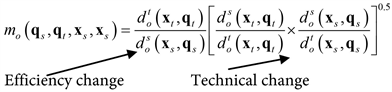
Figure 1 illustrates the two decompositions.

$\text{Efficiency change}=\frac{q_t/q_c}{q_s/q_a}$ (5)

$\text{Technical change}={\left[\frac{q_t/q_b}{q_t/q_c}\times \frac{q_s/q_a}{q_s/q_b}\right]}^{0.5}$ (6)

Equations (5) and (6) depict the distance functions being used by the actual distances being measured in the two decompositions also shown in the graph.

The following is the equation for input-orientated Malmquist productivity index

$TFPC={\left[\frac{d_s\left(q_s,x_t\right)}{d_s\left(q_t,x_t\right)}\frac{d_t\left(q_s,x_s\right)}{d_t\left(q_t,x_t\right)}\right]}^{0.5}$ (7)

For a technology that exhibits constant returns to scale output-orientated and input-orientated Malmquist indexes are exactly the same. Another interesting property of the index is that if panel data on input and output quantities are available then one can do away with the need for data on prices.

4. Link between Barnett’s Production Function of Banks and Malmquist Index for Productivity

Aggregation theory and index number theory both play a valuable role in measuring technical change. In the following is a brief account of some of the main results in the literature, on measuring banking industry technical change.

When technical change is possible, the financial intermediary’s production function is

$M_t^b=g\left({\alpha }_t,t\right)$ (8)

Figure 1. Malmquist index decomposition.

where α_t is the vector of factor inputs, namely labor, capital and materials as outlined in Barnett’s production process for banks. And

$M_t^b=f\left({\mu }_t;k_t\right)$ (9)

is the exact economic quantity aggregate over monetary assets μ_t, which includes outputs namely transaction deposits savings and time deposits. The technical change in the production of aggregate monetary output is equal to a shift in technology given in Equation (1) above, over time, so the right hand side of the equation has time as an argument.

Ohta (1974) defines the rate of change of total factor productivity as:

${\partial \log g\left({\alpha }_t,t\right)/\partial t|}_{{\alpha }_t}$ (10)

This measures the rate of disembodied technical change.

In case of neutral technological progress Equation (8) can be written as

$M_t^b=\Phi \left(t\right)g\left({\alpha }_t\right)$ (11)

where variations in Φ(t) produce parallel translations of isoquants. Then in discrete time the log change of this equation is the rate of disembodied technical change according to Ohta’s definition:

${\left(\log M_{t+1}^b-\log M_t^b\right)|}_{{\alpha }_t}=\log \left(\Phi \left(t+1\right)/\Phi \left(t\right)\right)$ (12)

By substitution of (11) in (12) we get

${\left(\log M_{t+1}^b-\log M_t^b\right)|}_{{\alpha }_t}=\log \left(M_{t+1}^b/M_t^b\right)-\log \left(g\left({\alpha }_{t+1}\right)/g\left({\alpha }_t\right)\right)$ (13)

Applying linear homogeneity to input or output aggregator function we get

$\log \left(g\left({\alpha }_{t+1}\right)/g\left({\alpha }_t\right)\right)=\log g\left({\alpha }_{t+1}\right)-\log g\left({\alpha }_t\right)$ (14)

and

$\log \left(M_{t+1}^b/M_t^b\right)=\log M_{t+1}^b-\log M_t^b$ (15)

where (14) and (15) can be measured by the discrete Divisia index over growth rates of input and output quantities respectively. Hence the rate of technological progress can be measured by the difference between two Divisia indices, one aggregating over growth rates of output quantities and the other over the growth rate of input quantities.

Caves, Christensen (1982) applied the same results to the case of non-homothetic g and f. They defined technical progress in terms of Malmquist input and output indexes. Furthermore, translog distance functions usage leads to measuring the rate of technological change in terms of Divisia input and output indices. This is the justification for using a proper production function in this paper for financial intermediaries i.e. Barnett’s function in the Malmquist index for productivity and nothing else. The kind of outputs a financial firm uses, connect its role to the transaction technology which is at the basis of the payment mechanism in the economy, only under this model. No other production function, except for this has satisfied all conditions for being amenable to calculations under the Malmquist index.

Barnett’s production function fulfills the following properties:

Separability of technology, confirmation to Aggregation theory (Barnett 1987).

1) Separability of technology: Aggregation over outputs is possible only if outputs are separable from inputs in the firm’s technology. This is referred to as “weak separability of the production function in the block of monetary components”. This is also of significance because Hicksian aggregation is not easy to satisfy aggregation over the firm’s joint monetary supplies μ_t. The existence of an output aggregate is shown in detail in Barnett 1987.

2) Confirmation to Aggregation Theory: Furthermore, once separability of the technology is established it is possible to apply the literature related to output aggregation to the case of multiproduct firms. This can then be used to aggregate over the produced monetary assets and to measure value addition and technological change in financial intermediation.

None of the two approaches i.e., the Production approach and Intermediation approach discussed earlier satisfy these properties, therefore Barnett’s production function is the best candidate in terms of input-output classification to be used in the Malmquist output and input indices.

Another reason why Malmquist should not be used with Accounting Approach stems from Valverde, Humphrey and Paso (2007) [14]. They warn against using the Malmquist index with the accounting-based approach. When the two are combined, index links the two sides of balance sheet output (assets) to inputs (liabilities) plus labor and physical capital. Because of the balance sheet constraint, which is also the accounting identity that equates the sum of asset (outputs) to the sum of liabilities (inputs). This identity makes efficiency measurement with this approach equivalent to a calculating a ratio of labor and capital inputs to asset value. This is erroneous and defeats the purpose.

Summarizing over the results and arguing in favor of the generalized production function we could say that:

● Distance functions completely characterize a production technology. (Fare 1988) [15]. It is possible to recover a technology from a distance function and vice versa. We have a proper production technology in case of Barnett’s production function, which obeys separability in inputs and outputs. This is not possible in case of Accounting based approaches.

● the rate of technological progress can be measured by the difference between two Divisia indices, one aggregating over growth rates of output quantities and the other over the growth rate of input quantities.

● Caves, Christensen (1982) generalized the same results to the case of non-homothetic input and output aggregators. In that case, technical progress is defined in terms of Malmquist input and output indexes. When the distance functions used to define the Malmquist indexes are trans-log, the rate of technological change is measured exactly in terms of Divisia input and output indices. This is in fact the nexus between Divisia index and the Malmquist index. Divisia index is actually a predecessor of the Malmquist index and this makes the case for an alliance between Malmquist index and Barnett’s Generalized Product ion function for financial intermediaries.

● The nature of financial firms’ outputs relates to their role in the transaction technology underlying the payment mechanism in the economy only under this model, which again qualifies the generalized function as the best candidate for measuring efficiency.

5. Literature Review

Research is filled up with several studies using accounting conventions to define inputs and outputs for a bank. There has never been even a single attempt to use economic theory-based definitions of a bank as in this paper. Table 4 summarizes the route research has taken over the years. The first column states the authors and year of publication, the second gives the title of the paper and third column summarizes the input-output classification used.

The following is a descriptive account of similar research based on accounting conventions:

Yang and Cao 2010 [22], examine the performance of seven of the largest Canadian Schedule 1 banks. They have used DEA analysis in order to calculate the efficiency scores for the Schedule 1 banks between 1998 and 2007. From these efficiency scores, Malmquist Productivity Index was used to calculate the productivity changes. They then compare the results with economic development in Canada within the research timeframe. Model sits well in comparison to general findings.

Asmild 2004 [23], calculate Malmquist index using DEA window analysis scores for Canadian top 5 banks. According to the calculations for both periods, Malmquist index and for all suggested definitions of same period frontier, the standard decomposition gives inappropriate results.

Berg et al. 1992 [9], used chained Malmquist indices in their paper. Results give evidence of regressive productivity growth before deregulation in the Scandinavian Banking industry but improved productivity after deregulation.

Vivas and Humphrey 2002 [24] talk about the bias in Malmquist index due to the technique applied in previous research studies. They are able to eliminate the bias when all output and inputs of the banking industry are used, rather than restricting the case due to unavailability of data or convenience of available data only.

Maniadakis and Thanasoullis 2004 [25], develop a productivity index. This can be used when producers cost minimize and know the input prices. The index is similar to the Malmquist index and has been extended to measure productivity. Productivity change has two components; efficiency and cost technical change. They furthermore, decompose aggregate efficiency change into technical and allocative efficiency change.

Worthington 1999 [26] uses nonparametric techniques to explore productivity

Table 4. Literature review various approaches.

of Australian banks by decomposing Malmquist index into technical efficiency change and technological efficiency change. This is carried out for a sample of credit unions. Post-deregulation evidence of efficiency change is observed.

Molyneux et al., 2004 [27], calculate parametric as well as non-parametric estimates of productivity change for European banks between 1994-2000. They use these approaches to identify structures that have benefited most and least from productivity change during the 1990s. Improvements in technological change are an outcome of productivity change. They also find that there is no appearance of catching-up by non-best practice institutions.

Grifell and Lovell 1997 [28] analyze the pattern of productivity change in Spanish banking from 1986-1993. The commercial banking sector and the savings banks sector dominate the banking industry. The paper examines productivity change separately for each sector and then also after merging them. According to the results commercial banks experienced a slightly lower rate of productivity growth, although a slightly higher rate of potential productivity growth. The reason was differences in managerial and institutional efficiency. Rate of technical progress, and also the adverse impact of diseconomies of scale in the commercial banking sector are some other reasons.

Tortosa-Ausina et al., 2008 [29], use DEA and bootstrapping techniques in order to explore productivity growth and productive efficiency specifically for Spanish savings banks from 1992-1998. Improvement in production possibilities have led to productivity growth as indicated by results. But average efficiency has remained quite constant over time. Bootstrap analysis however, is not statistically significant and it reveals that the disparities in the original efficiency scores of some firms are decreased to a huge degree.

Zeleneyuk 2006 [30], further elaborates on the work of Färe and Zelenyuk, 2003 [31] in which they use a theory to look for a method of aggregating Malmquist Productivity Index over units, which could be firms or countries. They further explore the aggregation of broken down components of the Malmquist Productivity Index.

Portela, Thanassoullis 2010 [32], work with negative data and come up with an index and an indicator of productivity. They use RDM (the range directional model). RDM is a particular case of the directional distance function, for calculating efficiency in case of negative data. This RDM can reflect productivity change, and it can also measure RDM inefficiency which can be used to result in a Luenberger productivity indicator. They also establish relationship between the two. This is called the meta-Malmquist index and meta-Luenberger indicator. They then show how the meta-Malmquist index can be both used to compare the performance of a unit over two time periods and the performance of two units in the same time period.

Pastor et al., 1997 [33], employ a non-parametric approach with the Malmquist index, to perform a comparison between efficiency, productivity and differences in technology of a subset of European and US banking systems for the year 1992.

Wheelock and Wilson 2003 [34], analyze the performance of U.S. commercial banks during 1984-2002. They measure performance relative to the maximum expected output and not relative to an estimated and difficult to measure boundary. Non-parametric Estimation with n-consistency is allowed because of this approach. It also avoids the usual curse of dimensionality that weakens traditional non-parametric efficiency estimators. The resulting estimates turn out to be robust with respect to outliers and noise in the data.

Alam 2001 examines US commercial banking industry in the 1980’s. The 80’s was an era of marked changes in the industry. Alam tries to answer the question if intensified competitive pressure which was generated by deregulation and notable financial innovations led to higher productivity during the 1980’s. To investigate this question, the paper uses the nonparametric Malmquist index. Paper finds a statistically significant productivity surge between 1983 and 1984. Post-1985, there was a regression in productivity and then the next two years sustained productivity progress was observed. Technological changes are the main reason for productivity changes rather than scale changes.

6. Data

The FDIC is the source of data for US Banks from 2006-2016. Detailed data on bank’s report of income and report of financial condition were used to extract input and output data. Outputs are checking deposits, savings and time deposits. Inputs are labor, materials and excess reserves. Rather than taking a sample of banks, all banks in the data in a given year are used in calculations. There are 5102 banks in the dataset for the year 2016. This number is larger for data from 2006, but as the industry passed through consolidation the number of banks dwindled. Below Table 5 gives a summary statistics of inputs and outputs used in this paper.

Table 5. Variable names, average and maximum values for all US Banks 2006-2016 (000’s of dollars).

7. Methodology

Table 3 represents the approach taken in this paper to define inputs and outputs of a bank. Table 1 on the other hand depicts the models used in Alam 2001. The two approaches are in stark contrast as accounting conventions are used in Table 1 to define inputs and outputs of a bank.

For this paper using inputs and outputs defined in Table 2 the Malmquist index is calculated as:

$\begin{array}{c}{m}_o\left(q_s,q_t,x_s,x_t\right)={\left[m_o^s\left(q_s,q_t,x_s,x_t\right)\times m_o^t\left(q_s,q_t,x_s,x_t\right)\right]}^{0.5}\\ ={\left[\frac{d_o^s\left(x_t,q_t\right)}{d_o^s\left(x_s,q_s\right)}\times \frac{d_o^t\left(x_t,q_t\right)}{d_o^t\left(x_s,q_s\right)}\right]}^{0.5}\end{array}$

R language has a package called “productivity” which enables calculation of Malmquist index for a bank for every two years in the time period considered. This process results in three scores for every bank, namely an overall Malmquist index efficiency score, a technical efficiency score and a scale efficiency score. Process is repeated for large banks separately which have a total asset size of more than $500 million.

8. Results

Table 6 gives the Malmquist index, average productivity scores for all banks in US from 2006-2016 and then for banks with asset sizes larger or equal to $500 million. Below is a graphic illustration of how the indices progress over time.

Figure 2 presents a comparison of average Malmquist productivity scores over the recent decade for all banks and large banks only. The average productivity for all banks lies below the 1.00 mark, which is in concordance with the estimates for efficiency from 80’s and 90’s, Berger, Hunter, and Timme (1993) [11].

Although values below 1.00 point towards a regression in performance as

Table 6. Malmquist index scores all banks and large banks only.

Figure 2. Malmquist over the years.

compared to earlier, but the average values are still very close to the cutoff point. There is a sort of smooth plateauing of the scores around the 0.985 mark, although the post-financial crisis era is also a part of this time period. Performance of large banks exceeding $500 million in total assets is showing some spikes and there are some points in time when they are able to touch the efficient cutoff point of 1.00. Large banks were more efficient as compared to all banks taken together.

Figure 3 is a depiction of 95% confidence intervals for Malmquist efficiency scores for all US banks. The confidence intervals also manifest the high efficiency value trend in the data.

Efficiency of banks:

Average efficiency scores are depicted in Table 7 and Figure 4. Efficiency scores highlight the within-the-frontier productivity of banks.

Efficiency has been rising overall for all banks, although falling short of the 1.00 mark. For this entire decade, overall efficiency has never touched 1.00. There is a slight upward trend in efficiency and overall the level is very close to 1.00, which means that even the financial crises didn’t dampen the performance of banks on average.

Large banks are even more efficient as we can see many years in the data, when large banks have shown 1.00 index score.

Figure 5 shows the 95% confidence interval range for all banks, which again is showing a trend towards the higher side.

Table 8 below gives technological scores for all banks and large banks.

Technological productivity:

Technology scores are slightly lower than the overall Malmquist scores and the efficiency scores alone. This is evident in Figure 6, scores for all banks mostly hover in the range of 0.97. Even large banks have shown slightly lower performance since the spikes as seen in the first two indices are not seen in case of technological productivity. But still technological productivity has also been quite high in the time period being studied.

Figure 3. 95% confidence intervals for Malmquist efficiency scores for all US banks.

Figure 4. Efficiency scores over the years.

Figure 5. 95% confidence interval range for all banks.

Table 7. Scale efficiency scores for all banks and large banks only.

Table 8. Technological index scores all banks and large banks only.

Figure 6. Technology scores over the years.

Figure 7 shows 95% confidence interval range of all banks technical scores which is also on the high side, although not as high as efficiency index ranges.

Reasons for persistence in index scores:

There could be a number of explanations of continued efficient performance of the US Banking sector. One of them is the fact that troubled banks are no longer in the population. Table 9 below gives the number of total banks in US over the years.

Figure 7. 95% confidence interval range of all banks technical scores.

Table 9. gives the total number of banks as reported by the FDIC over the years.

Banks with trailing efficiency levels being no longer a part of the population could be a reason for persistence in high efficiency scores into the 2000’s and beyond. Increased consolidation could be another reason, this can be observed by looking at the trend in the total number of branches and detailed record of M&A’s.

Secondly, Wheelock and Wilson 2017 [22], results for economies of scales of the US Banking sector also highlight a continued reaping of increasing returns to scale by the banking sector and this is especially applicable to larger banks. The same conclusion can be found in the case of productivity and scale and technological efficiency.

To further explore reasons for high efficiency, I run a panel regression of Malmquist index scores on a set of efficiency correlates. These efficiency correlates are also based on Barnett’s generalized model of production for banks. The following Table 10 illustrates the broad categories of correlates in the first column, traditional ratio measures used in the existing literature in the second column and correlates for Barnett’s generalized function in the third column.

Table 10. Efficiency correlates.

$\begin{array}{c}{\text{Malm}}_{it}={\alpha }_i+{\text{GDP}}_t+{\beta }_1{\text{Dep}}_{it}+{\beta }_2{\text{NI/input}}_{it}+{\beta }_3{\text{TC/dep}}_{it}+{\beta }_4{\text{Dep/excess}}_{it}\\ +{\beta }_5{\text{Dep/labor}}_{it}+{\beta }_6{\text{Dep/mat}}_{it}+{\beta }_7{\text{Exp/emp}}_{it}+{\beta }_8{\text{Atm}}_{it}+{\epsilon }_{it}\end{array}$

Above equation illustrates the fixed effects regression being used. Where ${\alpha }_i$ is the term for unobserved fixed effects across banks. GDP_t is specific to the time period of observation; it represents any change over time that affects all observational units in the same way. In this case it is the economic environment. We are considering the time period from 2011-2016, i.e., 5 years of observations for all banks in US in a given year. This creates an unbalanced panel of 38633 banks.

Dep_it is total deposits for i^th bank in t^th year.

NI/input_itis the net income to inputs of production ratio for i^th bank in t^th year.

TC/dep_it is the Total cost to total deposits ratio for i^th bank in t^th year.

Dep/excess_it is the Deposits to excess reserve ratio for i^th bank in t^th year.

Dep/labor_it is the total deposits to labor ratio for i^th bank in t^th year.

Dep/mat_it is total deposits to material ratio for i^th bank in t^th year.

Exp/emp_it is total expenses to employees ratio for i^th bank in t^th year.

Atm_it is Atm expense for i^th bank in t^th year.

Table 11 below is a fixed effects regression of Malmquist index on efficiency correlates.

Besides economic environment, efficiency scores are significantly affected by the risk management ratio, cost management ratio, and structure of funding.

Under risk management, Net income to inputs of production ratio was used. This is an efficiency ratio of inputs to production. Significant results for this correlate would mean higher input efficiency leads to better risk management, and therefore higher Malmquist efficiency index.

Cost management is measured in terms of deposits to excess reserve ratio, deposits to labor ratio and deposits to materials ratio. Deposits to excess reserve and deposits to material ratio both significantly affect Malmquist efficiency scores.

Table 11. Fixed effects regression of Malmquist index on efficiency correlates, US Banks panel data 2011-2016.

Signif. codes: 0 “***” 0.001 “**” 0.01 “*” 0.05 “.” 0.1 “ ” 1; Unbalanced Panel: n = 7405, T = 1 - 6, N = 38,633; Total Sum of Squares: 4.7608e+11; Residual Sum of Squares: 4.7324e+11; R-Squared: 0.0059708; Adj. R-Squared: −0.23006. F-statistic: 20.8359 on 9 and 31219 DF, p-value: <2.22e−16.

Table 12. One way (individual) effect between model.

Signif. codes: 0 “***” 0.001 “**” 0.01 “*” 0.05 “.” 0.1 “ ” 1; Total Sum of Squares: 2.6492e+11; Residual Sum of Squares: 4.4496e+10; R-Squared: 0.83204; Adj. R-Squared: 0.83184; F-statistic: 4070.36 on 9 and 7395 DF, p-value: < 2.22e−16.

Better management of excess reserves and material resources in order to generate more deposits leads to higher efficiency for banks.

Bank size as measured by total deposits is not a significant correlate, and this is also evident in large US banks just being slightly better in performance in comparison to all banks.

Technology measures such as ATM expenses do not significantly affect the efficiency index. Expense per employee ratio is not a significant factor, which means banks are not displaying expense preference behavior.

To improve the goodness of fit of the model a “between” regression was also run, Table 11 illustrates the results of the regression.

Table 12 gives the results of the one way (individual) effect Between Model.

The “between” regression immensely improves the R-squared and Adjusted r-squared values. Not only that but except for total deposits and ATM expenses all efficiency correlates turn out to be statistically highly significant.

9. Conclusions

In this paper, a different approach for defining bank inputs and outputs; namely Barnett’s generalized model of production for financial intermediaries was used to calculate the Malmquist productivity index and its components. This approach is based on economic theory model of banks as a firm. Previous research has only focused on accounting definitions of input and output of banks.

Results show a continuing trend in higher productivity for the entire banking sector, especially large banks. Within frontier efficiency has hovered in the high range of 0.985 which amounts to an average inefficiency of 1.5%, which is quite remarkable, especially after the financial crisis. Technological productivity, which measures how much further the frontier has been pushed, also continued to experience high scores, although slightly lower than scale efficiency. The reasons for continued high performance of the banking sector are mainly: cleansing up of the system post financial crisis and further consolidation being observed in the industry. Among the efficiency correlates, better risk management, cost management and improved structure of funding are some reasons for high efficiency of banks, based on Barnett’s generalized model of production.

Conflicts of Interest

The authors declare no conflicts of interest regarding the publication of this paper.

References

[1]	Barnett, W.A. (1987) The Microeconomic Theory of Monetary Aggregation. In: Barnett, W.A. and Singleton, K.J., Eds., New Approaches in Monetary Economics, Cambridge University Press, Cambridge, 115-168. Reprinted in Barnett, W.A. and Serletis, A., Eds., (2000) The Theory of Monetary Aggregation, North Holland, Amsterdam, Chapter 3, 49-99. https://doi.org/10.1017/CBO9780511759628.007
[2]	Wheelock, D.C. and Wilson, P.W. (2007) Robust Non-Parametric Quantile Estimation of Efficiency and Productivity Change in U.S. Commercial Banking, 1985-2004. Federal Reserve Bank of St. Louis, St. Louis, Working Paper No. 2006-041B. https://doi.org/10.2139/ssrn.912292
[3]	Sealey, C. and Lindley, J. (1977) Inputs, Outputs, and the Theory of Production and Cost of Depository Financial Institutions. Journal of Finance, 32, 1251-1266. https://doi.org/10.1111/j.1540-6261.1977.tb03324.x
[4]	Alam, I.M. (2001) A Nonparametric Approach for Assessing Productivity Dynamics of Large U.S. Banks. Journal of Money, Credit and Banking, 33, 121-139. https://doi.org/10.2307/2673875
[5]	Hancock, D. (1985) The Financial Firm: Production with Monetary and Nonmonetary Goods. Journal of Political Economy, 93, 859-880. https://doi.org/10.1086/261339
[6]	Barnett, W.A. and Jeong, H.H. (1994) Financial-Firm Production of Monetary Services: A Generalized Symmetric Barnett Variable-Profit-Function Approach. Journal of Business and Economic Statistics, 12, 33-46. https://doi.org/10.2307/1391922
[7]	Caves, D., Christensen, L. and Diewert, W.E. (1982) The Economic Theory of Index Numbers and the Measurement of Input, Output, and Productivity. Econometrica, 50, 1393-1414. https://doi.org/10.2307/1913388
[8]	Sherman, H.D. and Gold, F. (1985) Bank Branch Operating Efficiency: Evaluation with Data Envelopment Analysis. Journal of Banking and Finance, 9, 297-315. https://doi.org/10.1016/0378-4266(85)90025-1
[9]	Elayasiani, E. and Mehdian, S.M. (1990) A Nonparametric Approach to Measurement of Efficiency and Technological Change The Case of Large U.S. Commercial Banks. Journal of Financial Services Research, 4, 157-168. https://doi.org/10.1007/BF00352569
[10]	Elyasiani, E. and Mehdian, S. (1992) Productive Efficiency Performance of Minority and Nonminority-Owned Banks: A Nonparametric Approach. Journal of Banking & Finance, 1, 933-948. https://doi.org/10.1016/0378-4266(92)90033-V
[11]	Elyasiani, E. and Mehdian, S. (1995) Measuring Technical and Scale Inefficiencies in the Beer Industry: Nonparametric and Parametric Evidence. Quarterly Review of Economics and Finance, 33, 383-408. https://doi.org/10.1016/1062-9769(93)90005-5
[12]	Ferrier, G.D. and Lovell, C.A.K. (1990) Measuring Cost Efficiency in Banking: Econometric and Linear Programming Evidence. Journal of Econometrics, 46, 229-245. https://doi.org/10.1016/0304-4076(90)90057-Z
[13]	Athanassopoulos, A. (1998) Multivariate and Frontier Analysis for Assessing the Market and Cost Efficiency of Large Scale Bank Branch Networks. Journal of Money, Credit and Banking, 30, 172-192. https://doi.org/10.2307/2601208
[14]	Valverde, S.C., Humphrey, D.B. and del Paso, R.L. (2007) Do Cross-Country Differences in Bank Efficiency Support a Policy of “National Champions”? Journal of Banking & Finance, 31, 2173-2188. https://doi.org/10.1016/j.jbankfin.2006.09.003
[15]	Fare, R. (1988) Fundamentals of Production Theory. Lecture Notes in Economics and Mathematical Systems, Vol. 311, Springer Berlin, Heidelberg. https://doi.org/10.1007/978-3-642-51722-8
[16]	Aly, H.Y., Grabowski, R., Pasurka, C. and Rangan, N. (1990) Technical, Scale, and Allocative Efficiencies in U.S. Banking: An Empirical Investigation. Review of Economics and Statistics, 72, 211-218. https://doi.org/10.2307/2109710
[17]	Barr, R.S., Seiford, L.M. and Siems, T.F. (1994) Forecasting Bank Failure: A Non-Parametric Frontier Estimation Approach. Recherches économiques de Louvain/Louvain Economic Review, 60, 417-429.
[18]	Bauer, P., Berger, A., Ferrier, G. and Humphrey, D. (1997) Consistency Conditions for Regulatory Analysis of Financial Institutions: A Comparison of Frontier Efficiency Methods. Finance and Economics Discussion Series, No. 50, Federal Reserve Board, Washington DC, 85-144. https://doi.org/10.17016/FEDS.1997.50
[19]	Vanden Eeckaut, P., Ferrier, G.D. and Kerstens, K. (1994) Radial and Nonradial Technical Efficiency Measures on a DEA Reference Technology: A Comparison Using US Banking Data. Recherches Economiques de Louvain, 60, 449-479. https://doi.org/10.1017/S0770451800004619
[20]	Barth, J.R., Lin, C., Ma, Y., Seade, J. and Song, F.M. (2010) Do Bank Regulation, Supervision and Monitoring Enhance or Impede Bank Efficiency? SSRN Electronic Journal. https://doi.org/10.2139/ssrn.1579352 https://ssrn.com/abstract=1579352
[21]	Chortareas, G., Kapetanios, G. and Ventouri, A. (2016) Credit Market Freedom and cost Efficiency in US State Banking. Journal of Empirical Finance, 37, 173-185. https://doi.org/10.1016/j.jempfin.2016.03.002
[22]	Yang, Z. and Cao, Y. (2010) Assessing Canadian Schedule I Banks Using DEA Window Analysis and the Malmquist Index. 2010 7th International Conference on Service Systems and Service Management, Tokyo, 28-30 June 2010, 1-6. https://doi.org/10.1109/ICSSSM.2010.5530262
[23]	Asmild, M., Paradi, J.C., Aggarwall, V. and Schaffnit, C. (2004) Combining DEA Window Analysis with the Malmquist Index Approach in a Study of the Canadian Banking Industry. Journal of Productivity Analysis, 21, 67-89. https://doi.org/10.1023/B:PROD.0000012453.91326.ec
[24]	Lozano-Vivas, A. and Humphrey, D.B. (2002) Bias in Malmquist Index and Cost Function Productivity Measurement in Banking. International Journal of Production Economics, 76, 177-188. https://doi.org/10.1016/S0925-5273(01)00162-1
[25]	Maniadakis, N. and Thanassoulis, E. (2004) A Cost Malmquist Productivity Index. European Journal of Operational Research, 154, 396-409. https://doi.org/10.1016/S0377-2217(03)00177-2
[26]	Worthington, A.C. (1999) Malmquist Indices of Productivity Change in Australian Financial Services. Journal of International Financial Markets, Institutions and Money, 9, 303-320. https://doi.org/10.1016/S1042-4431(99)00013-X
[27]	Goddard, J. and Wilson, J. (2004) The Profitability of European Banks: A Cross-Sectional and Dynamic Panel Analysis. Manchester School, 72, 363-381. https://doi.org/10.1111/j.1467-9957.2004.00397.x
[28]	Grifell-Tatjé, E. and Lovell, C. (1997) The Sources of Productivity Change in Spanish Banking. European Journal of Operational Research, 98, 364-380. https://doi.org/10.1016/S0377-2217(96)00353-0
[29]	Tortosa-Ausina, E., Grifell-Tatjé, E., Armero, C. and Conesa, D. (2008) Sensitivity Analysis of Efficiency and Malmquist Productivity Indices: An Application to Spanish Savings Banks. European Journal of Operational Research, 184, 1062-1084. https://doi.org/10.1016/j.ejor.2006.11.035
[30]	Zelenyuk, V. (2006) Aggregation of Malmquist Productivity Indexes. European Journal of Operational Research, 174, 1076-1086. https://doi.org/10.1016/j.ejor.2005.02.061
[31]	Färe, R. and Zelenyuk, V. (2003) On Aggregate Farrell Efficiency Scores. European Journal of Operational Research, 146, 615-620. https://doi.org/10.1016/S0377-2217(02)00259-X
[32]	Portela, M.C. and Thanassoulis, E. (2010) Malmquist-Type Indices in the Presence of Negative Data: An Application to Bank Branches. Journal of Banking & Finance, 34, 1472-1483. https://doi.org/10.1016/j.jbankfin.2010.01.004
[33]	Pastor, J., Pérez, F. and Quesada, J. (1997) Efficiency Analysis in Banking Firms: An International Comparison. European Journal of Operational Research, 98, 395-407. https://doi.org/10.1016/S0377-2217(96)00355-4
[34]	Wheelock, D.C. and Wilson, P.W. (2017) The Evolution of Scale Economies in U.S. Banking. Revised Edition, Federal Reserve Bank of St. Louis, St. Louis, Working Paper 2015-21C.