How a Company Could Benefit from the Volatility of Prices: The Shipping Industry as a Case Study ()
1. Introduction
The wild volatility, though sporadic3, cannot be anticipated. Its mild version has been studied extensively by Statistics and Modern Finance. In practice, the following language to describe it has been used (Table 1).
Statisticians defined volatility as a yardstick of risk, emerging when “a variable (e.g., a price) moves certain distances, (counted by standard deviation), away from its average value in population”! In other words, the mean is the most probable outcome in large populations, as discovered by probability scientists
![]()
Table 1. The main uses and properties of volatility.
Source: author.
long ago, namely Laplace (1749-1827) and Gauss (1777-1855). More important and more recent (in 2008) is that volatility is distinguished, by Mandelbrot & Hudson (2006), into 3 states: mild, slow and wild.
2. Aim and Structure of the Paper
The prime aim is to supplement theory, which measured volatility—as an exclusive synonym of risk. Our line of thought is that volatility provides excellent opportunities, especially for Shipowners. Our secondary aim is to show that modern finance provides additional tools11,12): α for risk and fat tails, the “Hurst exponent”-H for cycles, the “Noah” effect for depressions and its alter ego, the “Joker”, for random catastrophes.
The paper is structured in 7 parts, apart from the literature review. Part I deals with the historical foundations of the “mild volatility”; Part II deals with the question of whether mild volatility is preferred by God. Part III deals with the anomalies that occurred in using mild volatility; Part IV deals with Normal Distribution in a closer investigation; Part V deals with the 3 business periods of the international shipowners (1741-2022, June). Part VI deals with the question of whether forecasting shipping volatility is possible. Part VII deals with the opportunities provided…by shipping volatility and how to exploit them. Finally, we conclude.
3. Literature Review
Mandelbrot (1963) discovered that the stock prices are “self-affine13”. He also found that the price changes follow a power law. Fama (1964) and Taleb (1997) argued that the “stock prices” move differently than what is supposed by “normal distribution”. They saw occasions of very large swings, following a “power law”, like…the earthquakes!
Liu et al. (1999), found that the “probability density function” of the volatility of the S&P500 was represented well by a “log-normal distribution”, but only it’s center. The tails were better represented by a power law, having an exponent, which is outside the “stable Levy” range. They used the “detrended fluctuations analysis”-DFA of 199414 & 199515, and the “power spectrum” analysis. DFA became popular16 in the next years, mainly among Asians.
Buchanan (2001) argued that if something follows the “bell” curve, then the numbers will cluster together and anyone beyond it will be extraordinarily unlikely (p. 45). He also argued that the 1929 crash was due to excessive borrowing. In 1997, the massive foreign debt collapsed the “tiger economies” of the S East. He also mentioned that research (since 1990) revealed that the sudden upheavals are likely, and perhaps inevitable (pp. 144-8)! Sornette (2003) (p. xv) wrote that the sudden transition from a quiet state to a crisis, is dramatic.
Stopford (2009) (p. 738-) explained why a worthwhile forecast could not be obtained in shipping: If the choice is to be “precisely wrong”, rather than be “vaguely right”. If one is about to forecast, but copies the past. If the present situation is good, there is pressure to produce more positive results (the herding instinct). The false consensus, coming from similar forecasts copying one another! Problematic model specifications and assumptions.
Lorange, Professor, and Shipowner, (2009), argued that anticipating the market swings17, (Figure 1), is a critical issue18.
As shown in Figure 1, the BDI from nearly 12,000 units in 2007 (last quarter), fell to 815 units in 2008 (4th quarter)—a disaster! This index is based on the current freight cost on various shipping routes, and is considered a barometer of the general dry shipping market. The index, after the start of the Russian invasion of Ukraine, increased to 2040 units on Feb. 28th, 2022.
Engelen et al. (2010) searched the “spot rate dynamics” of the VLCCs using “MDFA” and “the Rescaled Range analysis” (where the Hurst exponent showed
![]()
Figure 1. Bulk freight rates, per quarter, 2004-2008, based on the “Baltic Dry Index”-BDI. Source: author; data from Lorange (2009).
persistence). Hopefully, they stated that “a predictive freight rates model can be built”?
Stiglitz (2011) argued that (p. 17) during a crisis an expansive monetary and budgetary policy has to be applied. Stiglitz, believing in Keynes (Goulielmos, 2018b)—as we do—for the 1929-1935 depression, etc. dealt with the end-2008 crisis in USA and elsewhere, concluding that markets must be, after all, controlled.
The National Commission (2011) of the USA argued that the end-2008 financial crisis was the greatest since Great Depression in 1929 (p. xv), where by 2011, 26m Americans lost their jobs, 4m families lost their homes, 4.5m faced mortgage problems, and about $11 trillion vanished from people’s wealth…!! The crisis could be avoided (!). Two failures occurred: (a) of the financial regulations & their supervision and (b) of corporate governance & risk management; excessive borrowing, risky investments & lack of transparency took place. The Government was un-prepared. A systemic breakdown of accountability & ethics took place. The mortgage-lending standards collapsed. A detrimental contribution of the “over-the-counter derivatives” was added. A failure of the credit rating agencies occurred.
Silver (2012) distinguished the stock market periods into 2: the one in 1950s, and the other, “fast track”, in 2008s. This duality, Sornette (2003) argued, shows that there is a “fight between order and disorder”. For Silver the market is irrational 10% of the time! Buchanan (2013) argued that the “power laws19” and the “fat tails” are important for proper risk management, and for assessing the likelihood of rare market upheavals with accuracy (p. 79). He argued (pp. 235-236) that Levy’s mathematical work is valid if the fat tails have an exponent between 0 and 2. Goulielmos (2018a) found the shipping α = 1.43.
Weatherall (2013) argued that Osborne (1977) and Samuelson (2000) excused Bachelier L in supporting the “Random Walk”, in his doctoral thesis20, because the “Paris stock market” showed a mild variation of the stock prices (pp. 206-7). Osborne (1977) argued that rather the stock returns are normally distributed. Mandelbrot (2006, with Hudson) stated that not only “normal”, but also “log-normal distributions” cannot capture the full “wildness” of financial markets.
Galbraith (2014), argued that the “fat tails” show that extreme events are more frequent. Authors needed the end-2008 “Global Financial Crisis” to declare…the end of the “Normal”. For Galbraith normality is, among 3 other reasons: to prevent the breakdown of law and ethics in the financial sector.
Jiang (2015) attempted to find more evidence against the random walk hypothesis, a product of his doctoral thesis (2010-2014) at Courant Institute. He applied his research on the “exchange-traded funds” in the USA market, 2016-2013. This market deals with bonds, commodities, currencies, equities and with certain economic sectors (natural gas). His results support what Samuelson said that financial markets are in general micro-efficient and macro-inefficient.
Zheng & Lan (2016) applied the “MDFA” to search the dynamic features of the “spot rates of tankers”, using the Hurst exponent, and the time-dependent one, as well as the V-statistic21. These markets are fractal. The handy-sized ships showed lower volatility, while the larger vessels were more volatile. Jiang et al. (2019) argued that the “multifractal analysis” provided powerful tools to understand the complex nonlinear nature of the time series, and they wished to review it with an emphasis on financial markets.
In summarizing, the end-2008 crisis left an indirect beneficial lecture in many volumes: “volatility in the economies is going to be more frequent, and wilder”. Decisive will be if the “multifractality” movement will provide an “efficient/effective forecasting model”.
4. Methodology
We applied to the shipping industry the analysis of those authors, who have dealt with “the fractal”22 view of the “financial turbulence” (Mandelbrot & Hudson, 2006). We did not use the GARCH model, which could not generate sufficiently fat tails to be able to model leptokurtosis, which is actually observed in the “financial asset returns” and in “shipping industry’s freight rates”.
We adopted the “Rescaled range analysis” (Appendix 1), meaning the “analysis of the standardized volatility” due to “Hurst-Mandelbrot”. We filtered the time series, preferably by the first logarithmic differences23 (optional). We estimated the exponent H by the regression as follows: log(R/σ) = log(c) + H log(n), where R stands for the range, σ for the (local) standard deviation, c is a constant, n stands for the number of observations, and H is a power law, taking values between 0 and 1. If H > 0.50 the series show persistence, having a long-term memory. Our innovation was to calculate α, from 1/H = α (footnote 45). If α is < 2, wild volatility is present and a non-normal distribution has to be applied (e.g., the one having α = 1.50).
Five forecasting methods have been available to us since 2000: the “local ordinary least squares”; the “local principal components regression”, the “local ridge lines”, the “radial basis functions” and “the kernel density estimation”. One has to select one of the above methods by keeping a number of known observations off and then “forecast” them… The most accurate method of the 5, should be applied.
One has also to experiment with the parameters involved like the time delay (set = 1 as a rule), the embedding dimension, the steps ahead to forecast, the number of the nearest neighbors, etc. (footnotes 47, 48, 49). Important is to select the right time series, meaning that if volatility is high from minute to minute (Scan 1) or from day to day or from week to week, or from month to month (Scan 2), then this calendar time has to be selected.
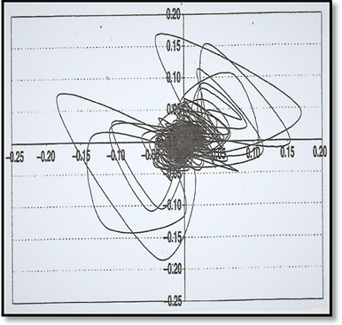
Scan 1. The attractor of the ASE, 1998. Source: Syriopoulos & Leontitsis in 2000.
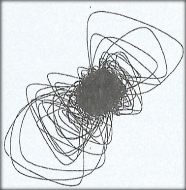
Scan 2. The attractor of shipping markets, 2006. Source: author.
From our experience forecasting the freight rates is like forecasting the “stock prices index” in the “Athens Stock Exchange”-ASE, unlike forecasting ship prices, which was most successful (not shown here).
As shown, the attractor24 of the “ASE price index”25 shows a concentration in its center, like a “basin of attraction”. From the 12,118 minus one observations, authors used the first 4000 in Scan 1. The created attractor, as shown, has a complex structure. The shipping attractor has nothing to be jealous of the stock exchange one!
5. Part I: The Historical Foundation of the Mild Volatility
5.1. The Law of Large Numbers
Established by the mathematicians etc. in 1834, (“Poisson’s law of large numbers”) (Mankiewicz, 2002). It is proved that the “expected mean” of a sample is equal to the mean of its population: E(msample) = μpopulation {2}, where m stands for the sample’s mean and μ for the population mean, given sample’s size n (Hogg & Craig, 1978). Also, the variance of the mean (of a sample) equals the variance (of its population) divided by the size of the sample: or σ2(mean) = σ2(population)/n {3}. This implies that the means of the samples concentrate round μ, as the size n (of the samples) increases.
5.2. The Central Limit Theorem26
“If a population has a variance σ2 and a mean μ, then the means of its samples will have a distribution approaching “normal”, with a mean m = μ, and a variance σ2/n, as n (the samples’ size) increases” (Brooks, 2014).
6. Part II: The Mild Volatility
The mild volatility describes life accurately during “normal” times. The probability P, of mild volatility of an x, is expressed by:
{4}
where x stands for the variable, μ stands for the mean, σ2 for the variance, σ for standard deviation and e27 and π are 2 mathematical constants. This was formed first by Laplace and applied to Statistics by Gauss. It gives the “probability of an event to occur, of a given population, under certain basic conditions28”. The key statement about {4} is given by Laplace: “Equation {4} gives the probability, which, however, can be a certainty (P(x) = 1)), if its ‘facts’ are ∞ repeated”! We see that both theorems, i.e., of the “large numbers” and of the “central limit”, require n → ∞. But, ∞ is an awkward (Judge et al., 1988) characteristic!
The graphical representation of {4} is as follows (Figure 2).
As shown, 68.2% of the outcomes are within ±1σ from the mean μ; 95.4% are within ±2σ and 99.6% are within ±3σ. Beyond ±3σ, the probability of an outcome is only ±0.2%. The distribution curve touches the horizontal axis (at zero). The curve is symmetrical.
More important are the 2 alternative distributions: the “Cauchy”, the “Financial” and the “Shipping” distributions (Figure 3).
As shown, the tails of the normal distribution stop at ±3σ. The financial distribution as well as the shipping one are between the other two, with alpha = 1.50. The shipping distribution, however is not symmetrical (Figure 4), as shown below.
As shown, the “shipping distribution” —fitted to 266 years (275-9), is not normal. More important is that it has a long tail on the RHS, a peak at 144 units (mean m > μ), and an alpha equal to 1.46 < 2 (not shown). The shipping standard deviation was 6.52σ away from its mean, in 2008 crisis as expected!
Important is that the normal (distribution) seems to expresses democracy and equitability. Everyone adds its value to the total, but the statistical outcome is determined by a (mathematical) law. No one can dictate anything to others (Mandelbrot & Hudson, 2006)! If there is a dictatorship, then a “Cauchy distribution” represents more accurately such a situation!
![]()
Figure 2. The normal distribution and the areas beneath it; their relation to σ. Source: unrecorded; modified.
![]()
Figure 4. “Maritime economics freight rates index” distribution, 1741-2015, vis-à-vis its normal distribution (1741 = 100 = 1947). Source: Data from Stopford (2009), amended; SPSS; skew: 3.2 (round.) > 0; kurtosis 13.7 (round.) > 3, giving a slimmer, long-tailed distribution with more weight in the center. Kurtosis, (showing a hump), is given by:
{6} for a variable Χ with a mean m.
7. Part III: The Anomalies Created in Applying the Mild Volatility
Research, till 1993, dealt exclusively with the mean (Brooks, 2014), representing, e.g. something very important for the investors: “the returns from their stocks”. In 1994, however, research created models concerning variance- also a traditional yardstick of risk. The risk was not always on the agenda, but as years passed-by, risk dominated in the analyses and international conferences, although there is no consensus about how risks, should be measured! The risks are at least two: the “Normal” and the “Wild”.
One econometric model, or rather a family of models, the GARCH29, with normal (0, 1, standardized) disturbances, used in almost every application since it has appeared. GARCH admitted that the variance σ2 varies with time, and this was a decisive step towards reality. In the past, certain models (& CAPM30) considered variance as constant! The physiology of the distributions, however, revealed a departure from normality: the leptokurtosis31.
Calvet and Fisher (2002) dealt with a “multifractal model in asset returns”, following their work in 1997 with Mandelbrot. This is a class of continuous-time processes, incorporating thick tails and volatility persistence. Variability is characterized by the Hurst exponent (Appendix 1). Returns vary by a power law of time. Moreover, the “GARCH-t” model32, also required constant fat tails over time (Brooks, 2014). The fat is measured by kurtosis, the 4th moment, based on the first 3 moments- the mean, the variance and the skewness:
{7}.
Alpha coefficient (Weatherall, 2013) deserves closer attention. Levy’s work (in 1937) on random processes, led him to a family of “stable” distributions. He found several33 between the “normal” and the “Cauchy”! In addition, wildness can be captured by α, which increases, as α → 0. The law of large numbers fails, and an average cannot be defined. An α between 1 and 2 permits the existence of the mean, but the variance is not well-defined! Risk, therefore, using σ is not possible to be measured.
The prices of cotton, which preoccupied Houthakker and mainly Mandelbrot (Mandelbrot-Hudson, 2006), had an α = 1.70. The most representative distribution for financial markets found the one with α = 1.50 (Weatherall, 2013). Shipping α found by Goulielmos (2018b) is equal to 1.43. Mandelbrot argued, in 1963, that volatility is ∞-except in the “normal” case.
Robbins and Coulter (2018) mentioned the opinion of one expert on weather, who said: “the pace of the change in our economy, and in our culture, is accelerating, and our visibility about the future is declining”. Also (p. 668), they argued that forecasting is less accurate, if the environment is rapidly changing, if there is a recession, if unusual occurrences happen, if discontinued operations exist and if one has to forecast one’s competitors.
8. Part IV: The Normal Distribution in a Closer Investigation
Jovanovic and Le Gall (2001) analyzed the work of Regnault J, in 1863, who constructed 2 models: one, which took the shape of the “random walk”—used by Bachelier in 1900- and the other dealt with the long-term speculation, asking if God practices the random walk…Others asked: if God plays dice (Stewart, Ian, in 1989, Blackwell). We ask: does God like symmetry?
The Normal distribution indicates that on average, and in the long term, a variable will reach its mean (known since 1809). This is also “stable”, meaning that its basic properties remain intact to any change. It is simpler than other L-stable distributions, requiring estimating only 2 parameters: the mean and the σ2. This is one reason to be preferred.
The “characteristic log function” of a general L-stable equation has 4 parameters:
α, β, γ and δ:
{8}.
Following Mandelbrot-Hudson (2006), the 4 parameters are: δ for location; γ for scale; β for skewness, and α for fat tails: 0 ≤ alpha ≤ 2! The normal distribution has α = 2 (no fat) and β = 0 (symmetry)34. For time series, the Hurst exponent H (Appendix 1) can show the existence of biased randomness if H > 1/2, indicating persistence (long-term memory). To derive Augustin Cauchy35 distribution’s characteristic function, we put α = 1 and β = 0 (symmetry) in {8}. The alternative parameter for risk is now α, which measures the volatility of a variable.
In Table 2, there are cases where Mandelbrot and Hudson (2006), and others, found normal distribution, historically, to fail.
As Mandelbrot & Hudson (2006) argued prices do not follow the normal distribution, and do not move independently, as required by the IID condition36.
9. Part V: The 3 Business Periods of the International Shipowners (1741-2022-June)
9.1. The Importance of the Shipping Industry
The shipping industry is important for serving seaborne trade. People will
![]()
Table 2. Cases where a variable moved away from μ by more than 3σ, and had an excess kurtosis.
Source: Mandelbrot & Hudson, 2006, pp. 95-98. (*) De Vries, (2001), pp. 3-6; as shown volatility increased in 2008 by 24%, 1% less than in 1929-1935! (**) Goulielmos (2009); (***) Goulielmos & Psifia (2007) A study of trip and time charter freight rate indices, 1968-2003, Maritime Policy & Management, Vol. 34, 1, pp. 55-67.
appreciate this more, in view of the coming “famine”, in 2022 and thereafter. Four nations were pioneers in this industry between 2011 and 2021 (UNCTAD): Greece, Japan, China and Singapore. Greece maintained the 1st position with 375m dwt (2021) and 417m dwt (2022). The value of the 4292 Greek-owned ships of $83b in 2018, increased in 2022, to 4766 ships and $159b (+almost 2 times37; and almost 1/2 of the blue economy of $361b). China increased its fleet from 2012-13 to 2016-2021. In 2013, Greece owned 243m dwt (22%); Japan 240 (21%); China 152 (14%), (Hong Kong 74m and Taiwan 48m); Germany 134 (12%); S Korea 69 (6%); USA 63; Singapore 52 and Norway 45m dwt.
The Covid-19 influenced shipping mainly in 2019-20 and in 2022, where major ports were closed (Shanghai in 2022). Also due to Russia-Ukraine war entire areas in Black Sea became not navigable for grain, corn oil, corn, steel. EU ban on Russian oil and gas had its own impact on all economies, including the oil and gas pipelines. Tankers transporting the USA oil reserves to EU undertook an important task, while containerships saw their own spring after certain winters. The Russia-Ukraine war, as any war before that, favors shipping during the war, and mainly after it, to rebuild the destroyed cities (Ukraine of 40m citizens).
9.2. Shipping: An Industry Where Entrepreneurs Have Learned to Live with Cycles
Stopford (2009) recorded 22 dry cargo shipping cycles, from 1741 (Figure 5), and till 2007, about 267 years, including also the 2 World Wars.
Stopford distinguished 3 cyclical periods: 1) the “sails”, from 1741 to 1871 (131 years), with the more beautiful ships (Scan 3).
2) The “tramps”38, from 1872 to 1947 (76 years), and 3) the “bulks”39, starting in 1947 (60 years to 2007). To this, we add the cycle that occurred in 2009 (10 years to 2018). The above 3 periods used apparently different technologies, including economies of scale, as well as higher speeds for the vessels. Up to 1960s, and even till 1985, the size of 10,000 dwt dry cargo ship dominated, (the “Liberty” ship), replaced by the modern bulk carrier 10 times larger (60,000 dwt).
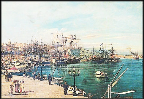
Scan 3. Sailing ships in port of Piraeus during 1800s. Source: Volonakis’ paint; modified.
Systemicity is the criterion for economists to deal with an economic phenomenon! So, volatility drew their attention when it became systemic. In the past, the business cycles were ignored, considered as having behavior like the weather. Economists were too proud to deal with “winds and waters”. When cycles re-occurred, economists dealt with them! But when growth theories41 prevailed, cycles were placed aside, till re-appeared in 1981-1987 (in dry cargoes) and in 2009-2018 (GFC)! Many theories exist for their causes; prevailing is that written by Keynes (1936).
The information about shipping cycles, however, is important, as e.g., Greek shipowners must know that their market’s volatility moves now, on average, in 8 years, and not in 15 years42, as experienced by their grand-fathers. Moreover, and more important, is that the good times, which lasted almost 6 years in the far past, last 3 years now, and the bad years are now 5! A dangerous assumption, we believe, comes from the shipowners43, who believe that shipping cycles last 744, or 8 years, with 3.5 - 4 years up and 3.5 - 4 years down!! Investments based on such unscientific basis are bound to fail nowadays, as in the past.
We all perhaps remember the case of “Sanko Shipping Co of Japan”, which put first all its eggs in one basket, (in tankers), and then put a massive order of 120 dry cargoes ships, in 1983, when tankers delivered losses, since end-1973. In 1981, 2nd half, also dry cargoes produced losses, till 1987 (1st half)! The Japanese company thought that the shipping cycle lasted 4 years, with absolute symmetry in its ups and downs (!), and thus the 1983 crisis, had to end in 1985 (Stopford, 2009). So, the company planned to get delivery of 120 ships, of about 30,000 dwt each, or 3.6m dwt, at the start of a boom!
Maritime history taught us, however, that the bad times are about 2/3 of the good times, as mentioned. Surely, the “secret shipbuilding policy” of the Japanese company, mentioned above, was revealed somehow to Greeks and the Norwegians. The substantial rise in Supply of over 13m dwt delayed the recovery further, and the prevailing trouph became deeper and longer, till 1987-1988! Figure 6 reminds us of the time differences between shipping peaks and troughs.
As shown, a trough may last long, and the fall in freight rates may be great. A peak may be short, and the increase in freight rates may be moderate. We analyze below the exact duration of the 21 shipping troughs (Table 3) after 1947.
![]()
Figure 6. One peak and 2 troughs in shipping. Source: author.
![]()
Table 3. Shipping troughs and their duration, 1746-2022.
Source: data from Stopford, 2009, p. 106; Napoleonic wars: 1792-1813; 1st World War, 1911-1913; 2nd: 1939-1946; Pandemic: 2019-2022; end-Feb. 2022: the Russian-Ukraine war.
9.3. Three Good Years Followed by 6 Bad Years
This pattern of 5 + 3 years shipping cycles reminded us of the “Joseph Effect” (Mandelbrot & Hudson, 2006). The Biblical story was symmetrical of 7 years up and 7 years down! God likes symmetry! Important is the relationship45 between alpha and the Hurst exponent H: α = 1/H (Peters, 1994). If α = 2, then H = 1/2 (normal distribution). The fat tails appear when α is < than 2 and equal to 1 (or lower) (→Cauchy distribution) and H = 1 (or lower). Shipping time series showed α = 1.43 (rounded), and H = 0.699986 (0.70 round.) > 0.50.
9.4. Nomikos et al. (2009)
They investigated the correct specification of volatility in Shipping. Their findings were mixed: FIGARCH, with log likelihood, did not work with Panamax and Cape (skewness increased); GARCH, etc. worked with less fat tails and kurtosis, but not for the Panamax; for the value-at-risk, GARCH failed in VLCC & Capes; FIGARCH failed in Suezmax/Aframax, and IGARCH failed in Panamax. FIGARCH better captured the dynamics and provided a better specification. The smaller ships showed persistent volatility?
Alizadeh & Nomikos (2011), searched the relationship between the dynamics of the “term structure” volatility and the “time-varying one46” of shipping freight rates, from 1992 to 2007, using “augmented EGARCH” models, and found it to be positive and asymmetric.
10. Part VI: Is Forecasting the Shipping Volatility Possible?
Goulielmos (2018a) tried to forecast the “shipping turbulence” from 2016 to 2035, using a Greek software47 and the “Kernel density function48” method. He found that the α shipping coefficient was equal to 1.43 (round.) for 277 years of freight rates of dry cargo ships, since 1750 (Figure 7).
![]()
Figure 7. α coefficients, 1750-2015 -actual - and forecast: 2016-2035. Source: Goulielmos (2018a); data from Stopford (2009), appendix C, supplemented for 2008-2015. First 9 years excluded by the program: starting from 1750; 8 years are missing, 1939-1946: starting from 1947; 1937-1938: data from S. Sturmey’s book on UK shipping & World competition (in 1962); α = 2 is the “normal” case.
As shown, there is a continuous fall in α after 1985, a peak year of the shipping depression (between 1981 and 1987). Thereafter, 15 years of troughs took place till 2018 (1998-2002; 2009-2018).
Table 3 explains Figure 7.
As shown, the shipping troughs lasted from 9 years to 6, on average, from 1741 to 2018.
Goulielmos (2018a), as mentioned, also forecast the index of the freight rates for dry cargo ships from 2016 to 2022 (Figure 8).
As shown, the forecasts of dry cargo freight rates for 2016-2022 were different than the actual! Especially in 2018-2019 and in 2021-2022 (March), when freight rates exploded. Goulielmos (2020) also predicted49 that a “Joker” would appear in 2022, and a shipping cycle, which started in end-2008, would last till 2018, as it did.
The “Joker”, is a term introduced by Peters (1994) to describe what happens in the market, which exhibits a persistent trend—identified by a Hurst exponent > 0.50—till an economic event occurs, which changes the existing bias either in magnitude, or in direction, or in both! The appearance of the Joker is a random event, and this was the GFC in end-2008. A Joker is also “the Russia-Ukraine war” in end-Feb. 2022.
The bad Joker, in the end-2008, brought a catastrophe in the dry cargo markets, till 2018. In 2020, a “good” joker appeared for a while and the market improved till 2022, after the Pandemic (Goulielmos, 2020). α in particular showed a lag, vis-à-vis the “freight rate dry cargo index”, of 3 years. The 2029-2030 period will show a trend towards a lesser wildness (α = 1.70), which, however, will not be sustained (Goulielmos, 2020).
![]()
Figure 8. Actual & forecast dry cargo shipping freight rates index, 2016-2022 (March) (1947 = 100). Source: author; data for grain freight rates in $, transformed into an index; forecasts from Goulielmos (2018a); The freight rates since 1986 refer to grain carried from US Gulf to Japan, via the Panama Canal (internet).
11. Part VII: The Opportunities Provided by Shipping Volatility, and How to Exploit Them
11.1. Does Volatility Increase Economic Inequality?
During the last crisis (2009-2018) some people came out of it richer! Certain authors wrote about this as an “increase” in global “economic inequality”. This proves that a crisis creates opportunities, but surely not for everybody! This paper asks why not for Greek shipowners?
11.2. Shipping: A Cost-Based Industry
The shipping industry is cost-based, and the shipowner who maintains the total cost of a vessel below the prevailing freight rate, he/she is efficient and effective. A capable shipowner knows that about 30% of the total cost of a vessel is due to her 2nd hand price. When the ship is new the capital cost increases to about 51% of the total cost (Figure 9), determined by the price paid to the shipyard.
As shown, the “capital cost” dominates the performance of a newly built tanker, and thus an efficient shipowner will try to minimize exactly this.
11.3. The Relationship between Ship Age and Her Price
What is the relationship between ship Age and her Price? Figure 10 shows this (Stopford, 2009) running a “regression” line between the two. The regression, fitted by the “least squares” method, was: P = 18.803 − 0.7337A, where P stands for price, A stands for age, a = 18.803 and b = 0.7337. Thus, a vessel (a Panamax) 10 years old got a price of $11.5 in 2002. In 2016 (March, 6th) her cost was $7.5m!
Companies, we believe, must run a regression for all vessels they own, as well for those to build, sell, buy, p.a., and try to have high correlation coefficients r, and n as large as possible. As shown, (red lines), certain prices went away from the regression line. Stopford did not mention what the variance was.
![]()
Figure 9. The composition of total cost for a newly built tanker. Source: data from Buckley, 2008, p. 369, supplemented.
![]()
Figure 10. The relationship of price and age of a specific type of vessel (Panamax) in 2002 (9 months data; n = 35). Source: Stopford (2009), p. 239, modified; r = ∑xy − nxmean ymean/nσxσy, where n = the number of pairs.
11.4. Do Shipowners Prefer to Buy Younger 2nd Hand Ships?
It is also apparent (Figure 10) the particular interest of buyers for younger ships, between 1 and 7 years of age, in 2002 (blue lines). This is a strategy also followed by Greeks, who bought ships 5 years old, by the majority. Α Cape 5 years of age provides almost 57.5% lower cost of capital ($47m new vis-à-vis $27m 2nd hand in early 2016).
One may be surprised by our persistence to suggest buying/building ships at rock-bottom prices, but this is the right strategy in an unpredictable world.
11.5. Ship Prices’ Volatility, 1986-1992
As shown, in 1990 (Figure 11 and Figure 12), a VLCC priced $42m (peak), and a 30,000 - 35,000-product tanker was priced ~$25m (peak), vis-à-vis 1986, when both were priced $7m! The volatility of these prices is high, and the question is what shipowners do? Owners of tankers ordered 15m dwt (7% of the total) at the end-1986 (correct), ~45m (21%) in end-1990 (very bad) and ~43m (20%) at the end-1992 (right)! In the bulk carriers’ sector, owners ordered 14m dwt (13%) in end-1986 (not shown, but correct), 17m (16%) in end-1990 (correct) and 37m (34%) dwt in 1991-2 (wrong), as prices went up (to $25m for a Panamax). So, shipowners did not fully exploit the volatility between 1986 and 1992!
11.6. Ship Prices’ Volatility, 1992-2008
Figure 13 presents the 2 main shipping markets -tankers and dry cargo- and the prices of 8 types of ships, 2nd hand and newly-built, in accordance with 3 characteristic ages.
As shown, the lower price range is included in the 2 vertical red lines, and, almost all, appeared in 2002-2003! So, a clever shipowner should have built/ bought ships then. To sell ships: worth noting is that all 8 types of vessels had a
![]()
Figure 11. Tanker prices of a VLCC, 10/12 years old & an oil product carrier, 5 years old, 1986-1992. Source: “Argo”-monthly shipping journal; Jan. 1993.
![]()
Figure 12. Bulk carriers’ prices, 5 years old, 1987-1992. Source: “Argo”-monthly shipping journal; Jan. 1993.
peak in their prices on 3 occasions: May 2005; Feb. 2008 and July 2008. What shipowners have actually done? We have data for 2007 (Figure 14).
As shown, global shipowners spent almost $6b in July 2007 (peak), and almost $37b for the entire year, to buy 1340 ships. However, they missed the month for low prices: May, 2006. The price then was $52m. The wrong timing cost $100m extra for a Cape 5 years old in end-2007! Thus, shipowners have to be trained to grasp opportunities created by volatility. In the shipbuilding market, the situation was as follows (Figure 15).
![]()
Figure 13. Prices of newly-built and 2nd hand ships of 3 types of dry cargoes and 5 types of tankers, 5, 10, and 20 years of age, 1993-2008. Source: Mpitsakis G., Naftica Chronica, 2008, pp. 72-80; modified.
As shown, 2007 was not the right year to build ships as prices were higher compared with just 1999. The lower prices occurred in 1964-1969, and in 1985.
Greeks spent $8.6bn on new buildings by mid-Oct. 2015 to build ships of 47m (round.) dwt vis-à-vis 48m (round.) dwt in 2014. Was this activity based on the idea that a shipping crisis has a 3.5-year-trough (2009-2012) and a 3.5 years peak (2012-2015)? If this was so then in 2015 the market should have recovered but it did not. One reason was the excess supply, as shown, till 2017 (Figure 16), the other was the fall in demand (seaborne trade).
As shown, the supply of the world tonnage, from 2000, increased from ~300m dwt to 600m (2 times) by 2011, and by 2017 increased to almost 900m (3 times). In the years 2000-2004, the increases were more conservative, but in 2009, and thereafter exploded, while the BDI fell to 290 - 330 units in 2016 vis-à-vis 11,793 in 2008! The shipowners are characterized by impatience, and when they see a price fall say 30%, they rush to order or buy, but prices continue to fall! Shipowners have only a 50% success for buying/ordering at rock bottom prices.
12. Further Research
We see the need to study the increased frequency of economic catastrophes and answer a number of questions (Table 4).
![]()
Figure 16. Expected tonnage supply worldwide, 2000-2017. Source: data from “Kathimerini” weekly newspaper, 06/03/2016.
![]()
Table 4. Why economic catastrophes emerge frequently?
(*) Economists, however, expelled time, as they work only in two dimensions- Supply, Demand → Price (Goulielmos, 2018c).
13. Conclusions
The CLT diverted the emphasis of scientists from the large numbers to normality51 (!), given that the CLT is related to a “normal” distribution—meaning the one covering the entire population52. The statisticians consider it more important than the law of large numbers. Brooks (2014) argued that it is well-known that stock markets (and freight rates markets, we add) are leptokurtic and tend to have longer lower tails. With small samples, the presence of outliers may also be more problematic!
Shipping is the industry where maritime economists attempt to predict the unpredictable. The catastrophic fall in dry cargo Baltic freight rates-index in 2008 was faster, steeper and longer than ever experienced. The same happened with a Panamax bulk carrier, where her earnings, from a high, in 2007-2008, of nearly 80,000 US$/Day, fell to about $14,000 in end-2008. Similarly, a Suezmax tanker earned during most parts of 2008 about $85,000/day, and in the end-2008 earned $30,000. A Cape earned $25,000 per day from 1980 to 2004 and $158,000 in 2008!
Greek shipowners have well-consolidated companies, so they have to become anti-cyclical by buying modern 2nd hand ships at depressed prices, and given their financial strength, they will have no need of the banks. This means exploiting volatility! A Cape dry cargo newly-built on 6th March, 2016, priced 47m, which is a price prevailing 12 years back (in 2004), but this was not as low as in 2002-2003 of $36m and in 2016 June of $32m!
For shipping, the “trough” years, since 1947 (Stopford, 2009), were 45 till 2018, meaning that the trouble years covered ~64% of the 70 years (1948- 2018), and not 10% as argued by Silver. Scientists had to revise their tools used to manage data—especially time series—to allow deviations from averages beyond 3σ, as a more frequent phenomenon of what their grandfathers experienced… Sad is that even the nonlinear chaotic methods of forecasting failed.
A certain theory demonstrated that there are 3 kinds of states dominating humanity: the mild, the slow and the wild (Mandelbrot & Hudson, 2006). The world created by humans, can be wild and the most wildness -as we all know- appeared in the Stock Exchanges more than once, while in end-2008 came this also from the Banks! In the life created by humans and by President Putin of Russia, even a…“3rd Global War” cannot be excluded.
Greek shipowners do not trust analysts53, as shouted out by G Procopiou on the occasion of the “Posidonia Maritime Exhibition” in 2016! When we provide to Greek ship-owners forecasts based on a mild market—which is not real, we prove ourselves unreliable, describing a world which does not exist Greek shipowners are right to shout out: “ignore the analysts”! This led us to suggest the following stratagems: to build ships, at rock bottom prices, as well larger than the ones owned; to buy ships at rock bottom prices larger and younger than the ones owned; to sell ships older and smaller than the ones bought. These stratagems serve 2 principles: “economies of scales” and “economies of age”, creating a lower capital cost and a competitive advantage. Depreciation is also lower.
![]()
Picture 1. A press statement of G. Procopiou, 2016. Source: Lloyd’s List, June 7th, 2016; modified.
As shown in Picture 1, Procopiou G suggested to Greek shipowners to buy ships in June 2016 and most importantly, to buy them at their lowest prices (rock bottom for us). He was right, as the 5 years old dry cargo Cape, on 6th March 2016, priced $27m; the Panamax $14m and the Supermax $12m, while in 2002-2003 the prices (Figure 13) of them were $32m and $16m for a Cape and a Panamax. Clarkson’s argued that the 2016 prices corresponded to those of 1999. Here is the opportunity! If prices were gradually rising or falling, in a moderate fashion, there could be no really a good opportunity! The mild volatility is not exciting and also not profitable! But to exploit the opportunities, one has to be prepared the $ way.
Appendix 1: The Rescaled Range Analysis
The range R is derived by subtracting from the maximum Y, the minimum Y. Range’s “rescaled” form is R/σn [5], dividing R by local standard deviation-σ. R gives also the distance travelled by a time series in time n. R coincides with d in Einstein’s formula (Table 1). We can generalize {5} to accommodate cases where d > and <
, following Hurst (1951): (R/σ)n = c * nH [6], where c is a constant, H is a power law, with a zero mean. Let us denote [6] in logs: log(R/σ)n = logc + H logn [7], where H moves in the interval [0 - 1]. Putting log(R/σ)n = d, logc = 1, H = 1/2 and logn = time, we derive Einstein’s formula {1}. Hurst (1951) estimated K = 0.73 > 0.50 for a wild volatility.
Ref.: Hurst, H.E. (1951). Long-term storage capacity of reservoirs, Transactions of the American Society of Civil Engineers 116: 770-799, 800-808. Steeb, W-H, (2015). The Nonlinear Workbook, 6th edition, World Scientific, Singapore.
NOTES
1Models constructed with constant variance over time.
2 Goulielmos (2009).
3The extent to which a series is (highly) variable over time, (usually measured by its standard deviation σ or variance σ2) (Brooks, 2014: p. 696).
4 Mandelbrot & Hudson, 2006, pp. 111-112.
5 Peters, 1994: volatility is pink, p. 275.
6 Peters, 1994, p. 275.
7 Goulielmos, 2018a; Mandelbrot & Hudson, 2006, pp. 111-122.
8 Peters, 1994, p. 275.
9 Peters, 1994, disputes this, p. 275.
10 Peters, 1994, p. 148-9. Black, F. & Scholes, M. (1973). “The pricing of options and corporate liabilities”, Journal of Political Economy.
11Except μ, σ2 and β (beta).
12Beta shows the amount by which a stock reacts to the market. If beta = 1.5 (very sensitive to the market/economy); the Treasury bills provide 2%; the market’s risk premium is 9%: the investor expects to gain: (1.5 × 9%) + 2% = 15.5% p.a., meaning: “the more one risks, the more one gains”. Its formula is: E(ri) = rf + βi(E(rM) − rf), where “the expected return r, on security i, equals the risk-free rate plus beta tines the market premium” (Mandelbrot & Hudson, 2006).
13 Mandelbrot (2002) defined similarity as a very special case of affinity. Mandelbrot & Hudson (2006) argued that the simplest fractals scale the same way in all directions = “self-similarity”. The fractals scaling in more than one direction are “self-affine”.
14Peng-Buldyrev-Havlin-Simons-Stanley-Goldberger in Physical review, E 49, 1684.
15Peng-Havlin-Stanley-Goldberger in CHAOS 5, 82.
16Cao et al., in 2018, published a book on “multifractal detrended analysis method” with applications in financial markets; a selection of papers.
17He (p. 33) argued that most of the global growth before 2008, stemmed from China.
18 Logothetis (2016) argued that for the last 25 years, before 2008, the “World Trade” grew 2 times faster, on average, than the “World GDP”, except in 2011. He admitted that shipping cycles of 7 years hold, on average! He proved wrong, however, with the BDI down to 471 units in end 2015… One explanation is the increased Supply by 757,609m dwt (2009-2015) (shown below). But also, the fall in demand, with especially the fall in coal imports by China for climatic reasons. All imports of grain, soyabeans, barley, corn, Nickel ore, increased (2015). China’s imports of iron ore from about 55 m tons in 1997 increased to 380m in 2007 and to 933m in 2014!
19Following Taleb (1997).
20“A theory of speculation”, in 1900, in French, published in Scientific annals of the “Higher Normal School”, 17, 21-86. Published in English by Cootner P H in 1964 in “Random character of stock market prices”, MIT Press.
21
, where R is the range and S the local standard deviation. A measure of stability.
22Fractal means broken. The parts, however, are affine to the whole. Chaotic systems often exhibit fractal behavior, but the 2 fields are intellectually distinct (Mandelbrot & Hudson, 2006: p. 261; M&H next). M&H defined fractal as a pattern, or object, whose parts echo the whole (p. 208). “Price-changes” can cluster in zones. M&H, p. 217, argued that their model represents a “fractional Brownian motion of multifractal time” of the “asset returns”. This modifies time, (as actual markets do; compressing and stretching it). The price is a function of the trading time and trading time is a function of clock time. This produces wild price fluctuations (big jumps & fat tails); & volatility clustering.
23If we have 2 equal observations and to avoid to get zero results, we add to the first e.g., 0001 (a very small decimal).
24An attractor defines the equilibrium level of a nonlinear dynamic system in a “phase space”. As shown, the attractor is made up by a substantial number of points (4000 in Scan 1). The interesting view here is that all points—except a number of initial ones (say n = 9)—tend to it asymptotically, as this could be shown by their trajectories for quite a number of initial conditions. Important is that the “phase space” is a mathematical space where time can take values −1 for the past, +1 for the future and 0 for the present!
25They belong to the units of the general index of the ASE, minute by minute, from 10.45 hours to 13.30, from 01/06/1998 to 10/09/1998.
26Having an independent and identically distributed random variable with expected mean m and variance σ2, the
converges to N(0, σ2), a random variable. Given a random sample of observations from an ∞ population, with any distribution, as long as it has a finite mean and variance, the function of the sample mean
has a normal limiting distribution (Judge et al., 1988: p. 86).
27e is a constant irrational number, with ∞ non-recurring digits, starting from 2.71828... Its origin is traced back to the early 17th c., when it found to be a useful part of the equations for calculating continuously compounded interest in finance (Mandelbrot & Hudson, 2006).
28The “reduced” Gaussian is derived if we put μ = 0 and σ = 1. The reduced Cauchy distribution is: f(x) = 1/π (1 + x2) {5} (“standard”).
29GARCH stands for the generalized (G), auto (A)—regressive (R), conditional (C), heteroscedastic (H) model, referring to a set of statistical tools to model the past data to vary. The term generalized stands for the model being more general than its progenitor, the ARCH (1982).
30The “Capital assets pricing model” states, in its simplest version, that the assets are priced in accordance with their relationship to the market (portfolio) of all…risky assets (based on betas).
31If “a time series shows a higher peak at the mean, and fatter tails, compared with normal distribution of the same mean and variance” (Brooks, 2014).
32The standardized errors are drawn from a “Student’s t distribution”.
33Using a generalized version of the central limit theorem (Peters, 1994). Peters (p. 199) argued that the stable Levy distributions are useful in describing the statistical properties of the turbulent flows, and 1/f noise, and are fractal. The idea of multifractality came from Mandelbrot in 1974 in the Journal “of fluid mechanics”. According to Olsen, Multifractal analysis. A selected survey, 2018, in internet), this analysis was revisited by physicists in 1986 by Halsey et al, in Physical review A, revealing the so-called “multifractal formalism”. In 1992 Cawley and Mauldin introduced into this formalism, the self-similar measures, in the “Advances in Mathematics” journal.
34An effective test for normality is the “Jarque-Bera” (in 1981) one, or the BDS (in 1996) for independence.
35A continuous probability distribution with undefined mean and variance studied in 1827 by Cauchy A (Kyle Siegrist http://www.randomservices.org/random/special/Cauchy.html.
36A sequence of random variables is independent & identically distributed, if each random variable has the same probability distribution as the others, and all are mutually independent (Clauset, 2015).
37The energy crisis and the R-U war had as a result for shipowners to build expensive ships like the LNGs.
38Ships destined to serve the trade having no prior destination or departure in a regular fashion.
39Today the Capes are ships of over 170,000 dwt.
The economies of scale nowadays have a larger impact than they used to have, not only on an average cost, but also on Supply, meaning that a ship of over 170,000 dwt (a Cape), coming into the market, or leaving it (scrapping40), is not without a greater influence.
40A serious amount of $s a shipowner may get by scrapping a large ship, meaning over $7m.
41Talking about cycles inevitably economists talked about “income distribution”, which was a controversial and political issue. However, talking about growth, everybody agreed, as the cake to be distributed would be larger and perhaps all people will get more! But they did not know that certain people will get the lion’s share!
42Near her end of economic life, having as much as 11 good years (1754-1764). Also, in 1988-1997… (=10 good years), but these were exceptions.
43G. Sarris, President Enterprises Shipping & Trading S A in “Naftica Chronica”, 2009, p. 32.
44 Logothetis (2016).
45Proof: let Rn be the sum of certain stable variables (in interval n); let R1 being their initial value, then: Rn = R1 * n1/α [1], stating that the sum of the n values scales by n1/α times initial value. Taking logs: α = logn/logRn − logR1 [2], and given that H = logR/S/logn [3], and if Rn − R1 is close to R/S, then 1/H = α [4]. α is also a measure of “fractal dimension”: = 2 − H. α is also related to βs, the spectral exponent: α = (βs – 1)/2.
46The “term structure” is related to the “standard deviation of freight rates at varying time horizons”.
47K. Syriopoulos -A. Leontitsis (2000), Software NLTSA (nonlinear time series analysis), 2.0 MS- DOS, C/C++, GNU CC 2.8 1988, RHIDE 1.4 1997, accepting 16,384 observations. “Chaos: analysis and forecast of time series”, Anikoula editions, Salonika, Greece (in Greek).
48Sugihara G & May R (1990). Nonlinear forecasting as a way of distinguishing chaos from measurement error in time series, Nature 344, pp. 734-740.
49A different method, the Radial Basis functions, was used. The coefficients chosen were: embedding dimension 5, time delay 1, relative vectors 16 and b = 1 following Casdagli, M (1989) Nonlinear prediction of chaotic time series, Physica D, 35, pp. 335-356, and the Greek software mentioned above.
50This affected all sectors of the economy for the last 30 years or so!
51 Judge et al. (1988), pp. 47-48.
52This is shown by
{9}.
53A giant Greek shipowner. His 3 companies, in end-2018, owned 15.2m dwt and 116 ships, in the 4th position, among 70 or so shipping companies of Greek ownership owning over 1m dwt. In 2022 May, he took over the “Skaramangas Shipyards” paying ~37m Euro!