Two Players Game Based on Schrödinger Equation Solution

Yijin Gao

Department of Mathematics, Iowa State University, Ames, USA.

DOI: 10.4236/tel.[phone]                

Abstract

Game theory between two no co-operation players is an important topic during these years. For each player, he has his own thoughts and for each time, maybe there is more than one idea in his brain which is a disturbance. It is really similar as the Schrodinger equation solution: for fixed time, the solution has different states in probability. In the paper, we connect these two things together and find the related topics between equilibrium and solution property.

Keywords

Game Theory, Schrödinger Equation, Evolution Process, Uncertainty Principle

1. Introduction

A physical or a socioeconomical system (described through quantum mechanics or game theory) is composed by n members (particles, subsystems, players, states, etc.). Each member is described by a state or a strategy which has assigned a determined probability ${\rho }_{ij}$. In evolutionary game theory, the system is defined through a relative frequencies vector x whose elements can represent the frequency of players playing a determined strategy. The evolution of the density operator is described by the von Neumann equation which is a generalization of the Schrödinger equation. It is a basic equation and a basic assumption of quantum mechanics proposed by Schrödinger, an Austrian physicist. So people started to use quantum language (entropy function) to study game theory (Orrell, 2019).

Firstly, Shubik (1999) finds there are three basic sources of uncertainty in an economy: exogenous, strategic, and quantum. The first involves the acts of nature, weather, earthquakes, and other natural disasters or favorable events over which we have no control. Strategic uncertainty is endogenous and involves our inability to predict the actions of competitors.

Later in their paper (Haven et al., 2018), they say in quantum mechanics, a state is formalized with a wave function, which is complex valued. That state will now form part of a Hilbert space. Position and momentum in quantum physics are real-valued, and one needs to find so called operators in the Hilbert space which can represent those real quantities. In Drabik (2011), the author introduces the basic concepts of quantum mechanics to the process of economic phenomena modelling. Quantum mechanics is a theory describing the behaviour of microscopic objects and is grounded on the principle of wave-particle duality. It is assumed that quantum-scale objects at the same time exhibit both wave-like and particle-like properties, but he just lists all the physics information, not exactly gives a connection with game theory.

These work (Hubbard, 2017; Hidalgo, 2007a, 2007b) focus on entropy (mostly is minmax question) to analysis the iteration of the game. But we want to analyze the game strategy based on Schrödinger equation solution (which also represents the state). We use the distance of two states to represent “good” or “bad” for two players and the “jump” between two different states is exactly the player’s strategy for the next game around (Samuelson, 1997).

Our paper concludes four sections, in the second section, we will give the model of Schrödinger equation and game theory separately. In third section, we give some basic theorems, examples and proof. In the last section, we have our conclusions and discussions.

2. Model

2.1. Schrödinger Equation

At the beginning of the twentieth century, experimental evidence suggested that atomic particles were also wave-like in nature. For example, electrons were found to give diffraction patterns when passed through a double slit in a similar way to light waves. Therefore, it was reasonable to assume that a wave equation could explain the behaviour of atomic particles. Schrödinger was the first person to write down such a wave equation. The eigenvalues of the wave equation were shown to be equal to the energy levels of the quantum mechanical system, and the best test of the equation was when it was used to solve for the energy levels of the Hydrogen atom, and the energy levels were found to be in accord with Rydberg’s Law.

In this part, we will give the exact Schrödinger equation, for simplifity, the system is closed which means two players can not be affteced by outside factors. So the potential can only change with people’s different thoughts. Also, each one can do optimal choices instead of information loss during their decision. The details will be discussed in the next sections.

Assumption 1. For a fixed time $t=t_0$ , for each player, they each only have two states, i.e., for player A, he has states $i_A$ and $j_A$ , similarliy, for player B, he has states $i_B$ and $j_B$ . And the states represents different solutions of the equation.

Assumption 2. For each player, they have their own same equation with different initial values. There is no entanglement between these two quantum phenomenon.

Schrödinger developed a differential equation for the time development of a wave function. Since the Energy operator has a time derivative, the kinetic energy operator has space derivatives, and we expect the solutions to be traveling waves, it is natural to try an energy equation. The Schrödinger equation is the operator statement that the kinetic energy plus the potential energy is equal to the total energy.

Traditionally, the Schrödinger equation is used to express the evolution of a quantum particle on the surface by its wave function $\varphi \left(x\mathrm{,}t\right)$ :

$\begin{array}{l}i\hslash \frac{\partial \varphi \left(x,t\right)}{\partial t}=-\frac{{\hslash }^2}{2m}{\nabla }^2\varphi \left(x,t\right)+v\left(x,t\right)\varphi \left(x,t\right),\left(t,x\right)\in \left(0,\infty \right)\times R,\\ \varphi \left(x,0\right)={\varphi }^0\left(x\right)\end{array}$ (1)

where $\nabla$ is the gradient operator at x, ${\nabla }^2$ is the Laplacian, m is the mass, $\hslash$ is the reduced Planck constant, $v\left(x\mathrm{,}t\right)$ is the real time-dependent potential, and ${\varphi }^0\left(x\right)$ is the initial wavefuntion.

But here we use this equation to express player’s choice moving and simplify the model as $m=\hslash =1$, the potential v is time-independent. Then the modified equation for player A changes to:

$i\frac{\partial {\varphi }_A\left(x\mathrm{,}t\right)}{\partial t}=-\frac{1}{2}\Delta {\varphi }_A\left(x\mathrm{,}t\right)+v_1\left(x\right){\varphi }_A\left(x\mathrm{,}t\right){\varphi }_A\left(x\mathrm{,0}\right)={\varphi }^0\left(x\right)$ (2)

Similarly, for player B, his equation is:

$i\frac{\partial {\varphi }_B\left(x\mathrm{,}t\right)}{\partial t}=-\frac{1}{2}\Delta {\varphi }_B\left(x\mathrm{,}t\right)+v_2\left(x\right){\varphi }_B\left(x\mathrm{,}t\right){\varphi }_B\left(x\mathrm{,0}\right)={\varphi }^1\left(x\right)$ (3)

Since the Schrodinger equation is like the “heat equation” (only difference is time t changes to it, so from the fundamental solution of heat equation, we know that there is also “fundamental solutions” for Schrödinger. After the comparsion, for the Schrödinger equation, we need the calculation of $\sqrt{i}$, which in one dimension situation. Actually the sqaure root of i has two roots which is suitable for our player’s two states in a time.

2.2. Game Theory

Game theory is a set of techniques to study the interaction of “rational” agents in “strategic” settings. Here “rational” measn the standard thing in economic: maximizeing the obejectives functions subject to conditions; “strategic” means the player care not only their own actions, but also about the actions taken by other player.

Modern game theory becomes a field of research from the work of John von Neumann. In 1928, he wrote an important paper about two-person zero-sum games. In 1944, he and Oscar Morgenstern published their classic book (Von Neumann & Morgenstern, 1947), Theory of Games and Strategic Behavior, theta extended the work on zero-sum games, and alsp started cooperative game theory. In the early 1950’s, John Nash made his contributions to non-zero-sum games (Nash Jr., 1950) and started bargaining theory. After that, there was an explosion of theoerical and applied work in game theory and the methodology was well along its way to its current status as a tool (Shubik, 1999; Samuelson, 1997; Selten, 1975; Samuelson, 2016).

And in our paper we will focus on noncooperative game theory, which means the former takes each player’s individual actions as primitives, whereas the latter takes joint actions as primitives. And we have the following assumptions about the players:

Assumption 3. The number of players is 2, player A and player B.

Assumption 4. There is no outside factors affecting their strategies.

Assumption 5. Each one is smart enough to have the optimal choice and no information loss when they have the decision. From the Schrödinger equation, The conservation law is true.

Definition 1. Players has no information loss during any time they make the decision is the $L^2$ norm integration of their “equation” solution from $-\infty$ to $\infty$ is always constant 1.

${\displaystyle {\int }_{-\infty }^{\infty }}{\left|{\varphi }_j\left(x,t\right)\right|}^2\text{d}x=1,j=A,B$

Since this integral must be finite (unity), we must have the solution $\varphi \left(x\mathrm{,}t\right)\to 0$ as $x\to \infty$ in order for the integral to have any hope of converging to a finite value. The importance of this with regard to solving the time dependent Schrödinger equation is that we must check whether or not a solution $\varphi \left(x\right)$ satisfies the normalization condition.

Definition 2. (Distance Between Different States). Distance between two state i and j is defined as:

$Dis\left(i\mathrm{,}j\right)={\Vert i-j\Vert }^2$

Definition 3. (Information of Strategy Sets). A collection of information set, I is a set of linear combination of two solutions for a fixed time $t=t_0$ , e.g. player A at time $t=t_0$ , his information set is:

$I=\left\{a\times {\varphi }_{Ai}\left(x\mathrm{,}{t}_0\right)+b\times {\varphi }_{Aj}\left(x\mathrm{,}{t}_0\right)\right\}$

Here ${\varphi }_{Ai}\left(x\mathrm{,}{t}_0\right)\mathrm{,}{\varphi }_{Aj}\left(x\mathrm{,}{t}_0\right)$ are the basic solutions of the equation. It is a mixed strategy for player A since he has two pure strategy distributions. $a\mathrm{,}b$ satisfying ${\left|a\right|}^2+{\left|b\right|}^2=1$. Just like the famous Schrödinger’s cat paradox which stated by Schrödinger in 1935. He presented a case of cat in a box which has fifty percent of survive and fifty percent it may die. So if we open the box, we can find the cat is alive or dead, but when we close the bos, there are infinity states it can be. According to this, we can explain the startegy: when we do the choice, we only have A and B these two choices. But when we are thinking, no one knows what we are thinking and actually we have infinity thoughts in our own brain.

Definition 4. (States Evolution as Strategy Change). When player A starts to change his strategy according to his guess of player B’s behavior, state change means the evolution for the Schrödinger solution. If his initial state is i, and the state changes to j after time t, the relation between i and j is

$j={\text{e}}^{iHt}i$.

Of course the time is a continuous parameter we obvious have

$\underset{t\to 0}{\lim }j=i$

Definition 5. (Strictly Dominant Strategy) Similiarly as the definition in traditional game theory, a startegy state $A_i$ is a strictly dominant strategy for player A is for all ${\bar{A}}_i\ne A_i$ , and all states $B_j$ for player B, $Dis\left(A_i\mathrm{,}{B}_j\right)<Dis\left({\bar{A}}_i\mathrm{,}{B}_j\right)$ .

Definition 6. A state i and j for A and B is a Nash Equilibrium if and only if their distance is the least, i.e., for any other states $i^{\prime }$ and $j^{\prime }$ , $Dis\left(i\mathrm{,}j\right)\le Dis\left(i^{\prime }\mathrm{,}{j}^{\prime }\right)$ . It also has another name: Stable Equilibrium.

Remark 1. This idea is from the model of the electron. The internal power between two electron is related to their distance, more closeness more power. If they are far away, exact little power between them, we do not care about these two electron. The two players are the “opponents” and “partner”, player A is affteced by B and player B is affected by A. So there should be more “power” between them.

Definition 7. (Uncertainty principle for player) Any player of two can not exactly guess what his opponent’s strategy in the next step for what probability.

Remark 2. The uncertainty principle is one of the most famous ideas in physics. It tells us there is a fuzziness about the behavior of quantum particles and we can not determine particle’s position x and momentum p at the same time. There is a famous inequality derived by Werner Heisenberg:

${\sigma }_x{\sigma }_p\ge \frac{\hslash }{2}\mathrm{.}$

where $\hslash$ is the reduced Planck constant: $\hslash /\left(2\pi \right)$. In two-players game, x represent their opponent’s behavior set (which is also the information set), p represets the related probability to take such decision. This phenomenon can not happen: player B continues his strategy always whatever A’s strategy is, then $\Delta x=\Delta p=0$, a contradiction with the uncertainly principle. In next section, we will give the example and proof about this.

3. Basic Theorem

Theorem 3.1. A player can have at most one strictly dominant strategy.

Proof. If we assume player A has two strictly domiant strategy and each one is state $i_1$ and $i_2$, then for any state $i_A\ne i_1$ and states j for player B, we have the inequality:

$Dis\left(i_1\mathrm{,}j\right)<Dis\left(i_A\mathrm{,}j\right)\mathrm{.}$

Same idea for state $i_2$, we still have the inequality:

$Dis\left(i_2\mathrm{,}j\right)<Dis\left(i_A\mathrm{,}j\right)\mathrm{.}$

We pick $i_A=i_2$ in the first inequality and pick $i_A=i_1$ for the second one, which is a contradiction. $■$

Remark 3. There can be no strategy state i for player A such that for all $\bar{i}$ of A and j of B, $Dis\left(i\mathrm{,}j\right)<Dis\left(\bar{i}\mathrm{,}j\right)$ . B is the same.

Theorem 3.2. The game system is closed under the time-evolution, which means $L^2$ norm of the state (solution) is always 1.

Proof. It is obvious from the property that ${\left|{\text{e}}^{iHt}\right|}^2=1$. $■$

Theorem 3.3. The time evolution operator is only related to its end time: intial time $t_0$ and ending time $t_1$ , it has no relation with the middle states from $t_0$ to $t_1$ . From the strategy idea, two players will have the decision in a fixed time and the opponent does not care about your thinking process.

Proof. Assume we have the inital state $i\left(t_0\right)$ and start to evolve to time $t_1$, there are two possibilities: 1) First one is directly “jump” from $t_0$ to $t_1$ ; 2) Second part we have many “stopping thinking time” $t_2\mathrm{,}{t}_3\mathrm{,}\cdots \mathrm{,}{t}_n$, until $t_1$. Compare these two states:

${\text{e}}^{iH\left(t_1-t_0\right)}{i}_{t_0}$

${\text{e}}^{iH\left(t_1-t_n\right)}{\text{e}}^{iH\left(t_n-t_{n-1}\right)}\cdots {\text{e}}^{iH\left(t_2-t_0\right)}{i}_{t_0}={\text{e}}^{iH\left(t_1-t_0\right)}{i}_{t_0}$

We find they have the same result and finish the proof. $■$

Theorem 3.4. Two players will get Ne (Nash Equilibrium) in a period time.

Proof. If we consider two players evolve separately, which means player A is from state j to state ${\text{e}}^{iH{t}_0}j$, and player B is from state i to state ${\text{e}}^{iH{t}_1}i$, then calculate their distance:

${\Vert {\text{e}}^{iH{t}_0}j-{\text{e}}^{iH{t}_1}i\Vert }^2={\Vert {\text{e}}^{iH{t}_0}\left(j-{\text{e}}^{iH\left(t_1-t_0\right)}i\right)\Vert }^2={\Vert j-{\text{e}}^{iH\left(t_1-t_0\right)}i\Vert }^2\mathrm{.}$ (4)

So we can only consider the state i evolution! Assume we evolve after time t, then the distance between these two is:

$\begin{array}{c}Dis\left(j\mathrm{,}{\text{e}}^{iHt}i\right)={\Vert j-{\text{e}}^{iHt}i\Vert }^2\\ ={\Vert j\Vert }^2+{\Vert i\Vert }^2-2Re\left(j{\text{e}}^{iHt}i\right)\\ =2-2Re\left(j{\text{e}}^{iHt}i\right)\end{array}$ (5)

which is function of t and we want to minimize the $Dis$, so need to make sure $Re\left(j{\text{e}}^{iHt}i\right)$ as big as enough. Now we write the state in the linear combination of energy eigenstate $E_p$ :

$j={\displaystyle \underset{p=1}{\sum }}{\alpha }_p{E}_p$

$i={\displaystyle \underset{p=1}{\sum }}{\beta }_p{E}_p$

And each constane ${\alpha }_p$, ${\beta }_p$ can be expressed as the norm times the exponential function of phase:

${\alpha }_p=\left|{\alpha }_p\right|{\text{e}}^{i{\omega }_p^1}$

${\beta }_p=\left|{\beta }_p\right|{\text{e}}^{i{\omega }_p^2}$

Then

$\begin{array}{c}j{\text{e}}^{iHt}i={\displaystyle \underset{p=1}{\sum }}{\alpha }_p{E}_p{\text{e}}^{iHt}{\displaystyle \underset{p=1}{\sum }}{\beta }_p{E}_p\\ ={\displaystyle \underset{p=1}{\sum }}\left|{\alpha }_p\right|{\text{e}}^{i{\omega }_p^1}{E}_p{\text{e}}^{iHt}{\displaystyle \underset{p=1}{\sum }}\left|{\beta }_p\right|{\text{e}}^{i{\omega }_p^2}{E}_p\end{array}$ (6)

For fixed p, $p=1$ situation:

$\begin{array}{c}\left|{\alpha }_1\right|{\text{e}}^{i{\omega }_1^1}{E}_1{\text{e}}^{iHt}\left|{\beta }_1\right|{\text{e}}^{i{\omega }_1^2}{E}_1=\left|{\alpha }_1\right|\left|{\beta }_1\right|{\text{e}}^{i{\omega }_1^1}{E}_1{\text{e}}^{iHt}{\text{e}}^{i{\omega }_1^2}{E}_1\\ =\left|{\alpha }_1\right|\left|{\beta }_1\right|{\text{e}}^{i{\omega }_1^1}{\text{e}}^{-i{\omega }_1^2}{\text{e}}^{i{E}_{j}t}\\ =\left|{\alpha }_1\right|\left|{\beta }_1\right|{\text{e}}^{i\left(E_{j}t+{\omega }_1^1-{\omega }_1^2\right)}\\ =\left|{\alpha }_1\right|\left|{\beta }_1\right|\left(\cos \left(E_{j}t+{\omega }_1^1-{\omega }_1^2\right)+i\sin \left(E_{j}t+{\omega }_1^1-{\omega }_1^2\right)\right)\end{array}$ (7)

Return back to Equation (6), we have the final formula:

$j{\text{e}}^{iHt}i={\displaystyle \underset{p=1}{\sum }}\left|{\alpha }_p\right|\left|{\beta }_p\right|\cos \left(E_{j}t+{\omega }_1^1-{\omega }_1^2\right)+i{\displaystyle \underset{p=1}{\sum }}\left|{\alpha }_p\right|\left|{\beta }_p\right|\sin \left(E_{j}t+{\omega }_1^1-{\omega }_1^2\right).$

To maximize the Equation (5) is equal to:

$\max Rej{\text{e}}^{iHt}i=\max {\displaystyle \underset{p=1}{\sum }}\left|{\alpha }_p\right|\left|{\beta }_p\right|\cos \left(E_{j}t+{\omega }_1^1-{\omega }_1^2\right)={\displaystyle \underset{1}{\sum }}\left|{\alpha }_p\right|\left|{\beta }_p\right|$

Since $\left|\cos \theta \right|\le 1$ for any $\theta$. Here we will use the following lemma to make sure we can take the equality for special t.

Lemma 3.5. There exists infinite $t\in \left[\mathrm{0,}\infty \right)$ such that $\cos \left(E_{p}t+{\omega }_p^1-{\omega }_p^2\right)=1$ for each p and the period time is related to $E_1$ and $E_2$ .

Proof. We focus on $p=2$, $\left(p>2\right)$ is the same extension.

Assume there exists two numbers $k_1$ and $k_2$ such that the following equalities satisfy:

$E_{1}t+w_1^1-w_1^2=2k_1\pi$

$E_{2}t+w_2^1-w_2^2=2k_2\pi$

If we rewrite these equations with t, we have the following equality:

$\left(2k_1\pi +{\omega }_1^2-{\omega }_1^1\right)E_2=\left(2k_2\pi +{\omega }_2^2-{\omega }_2^1\right)E_1$

$2k_1{E}_2\pi +\left({\omega }_1^2-{\omega }_1^1\right)E_2=2k_2{E}_1\pi +\left({\omega }_2^2-{\omega }_2^1\right)E_1$

$k_1{E}_2-k_2{E}_1=\frac{\left({\omega }_2^2-{\omega }_2^1\right)E_1-\left({\omega }_1^2-{\omega }_1^1\right)E_2}{2\pi }$

$k_1=\left(k_2+\frac{{\omega }_2^2-{\omega }_2^1}{2\pi }\right)\frac{E_1}{E_2}-\frac{{\omega }_1^2-{\omega }_1^1}{2\pi }$

Obviously we can choose suitable ${\omega }_1^1\mathrm{,}{\omega }_1^2\mathrm{,}{\omega }_2^1\mathrm{,}{\omega }_2^2$ such that their difference is

some integer q times $2\pi$, according from the famous Bohr formula: $E_n=\frac{E_1}{n^2}$, so $\frac{E_1}{E_2}$ is the rational expression $\frac{n_1^2}{n_2^2}$, pick suitable $k_2$ such that $k_1$ is also an

integer. Then go back to the t equation to get t. Simliarly, for $p>2$, we can still find their least common multiple. $■$

Example 1. (For Definition 7) The prison’s dilemma is a standard example of a game analyzed in game theory and we will use it first as an example for the uncertainty.

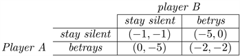
1) If A and B each betray the other,each of them serves two years in prison;

2)If A betrays B but B remains silent,A will be set free and B will serve three years in prison (vice versa).

3)If A and B both remain silent,both of them will serve only one year in prison.

So actually each player is in the dilemmas and no one knows his/her opponent’s strategy for the next step. It is a classical application of the “Uncertainty Principle”.

Example 2. (This example is from the lecture notes (Ferguson, 2005) (Odd and Even) Player A and B simultaneously call out one of the numbers one or two. Player A’s name is Odd; he wins if the sum of the numbers is odd. Player B’s name is Even; she wins if the sum of the numbers is even. The amount paid to the winner by the loser is always the sum of the numbers in dollars. We choose $X=\left\{1,2\right\},Y=\left\{1,2\right\}$ and the table is following:

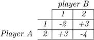
Let us analysis the game from Player A’s point of view.Suppose he calls “one”3/5ths of the time and “two”2/5ths of the time at random.In this case,

1)If B calls “one”,A loses 2dollars 3/5ths of the time and wins 3dollars 2/5ths of the time;on average,he wins 0.It is a even game in the long run.

2)If B calls “two”,A wins 3dollars 3/5ths of the time and loses 4dollars 2/5ths of the time and average he wins 1/5.

Clearly if A mixed his choices in this given way,the game has two ending:even or A wins 0.2dollar on the average every time.

1)If we think about after a long time “even”,A and B have no change,without loss of generality,the schedule for A is 1,1,1,2,2.Then B starts to think if he can do some change and earn money.So when A is “asleep”,she chooses 2when A is 1and she chooses 1when A is 2.Then each time she can earn 3dollars,A is losing! So based on such situation happen,A should be clear each step and do some changes which is hard for B to guess A’s strategy.

2)Similarly,for second situation.B calls “two”and A wins 0.2dollar average time.A is happy since he can earn money without doing any change,but B want to “save”money unless each game she will lose 0.2average.So she will call “one”without any dilemma,at that situation,A get nothing (since the average payoff is 0),so he will try to make some changes.In that case,each one will behave randomly without fixed strategy.

It satisfies the uncertainty principle.

However, player A can not player know B’s strategy, can he guess her probability for the next step? Of course he can, this is the following theorem from the quantum mechanics.

Theorem 3.6. For player A, he can guess the probability of player B’s from state $j_1$ to $j_2$ at time t:

$P_{j_1\to j_2}\left(t\right)={\left|C_2\left(t\right)\right|}^2$

Here $C_2\left(t\right)$ is definded as:

$C_2\left(t\right)=-i{\displaystyle {\int }_0^t}{H^{\prime }}_{21}\left(t^{\prime }\right)\exp \left(i{\omega }_0{t}^{\prime }\right)\text{d}{t}^{\prime }$

$H^0$ is the initial Hamiltoian operator: $-\frac{1}{2}\Delta +v_1$. The player A has a time dependent perturbation $H^{\prime }\left(t\right)$, and ${H^{\prime }}_{12}=j_1{H}^{\prime }{j}_2$, ${H^{\prime }}_{21}={\left({H^{\prime }}_{12}\right)}^{\mathrm{<mo>\; *\; </mo>}}$, ${\omega }_0=\frac{E_2-E_1}{\hslash }=E_2-E_1$. We write $H=H^0+H^{\prime }\left(t\right)$.

The proof is similar from the reference book (Griffiths, 2007).

Proof. To begin with, let us suppose that thare are just two states $j_1\mathrm{,}{j}_2$, then the solution function $\varphi \left(t\right)$ can be expressed by the combinations of these two:

$\varphi \left(t\right)=C_1\left(t\right){\varphi }_1{\text{e}}^{-i{E}_{1}t}+C_2\left(t\right){\varphi }_2{\text{e}}^{-i{E}_{2}t}\mathrm{.}$

And now since we have the perturbation, the new Schrödinger equation is:

$H\varphi =i\frac{\partial \varphi }{\partial t}$

Then combine these two together and cancel the term, hence

$C_1\left[H^{\prime }{\varphi }_1\right]{\text{e}}^{-i{E}_{1}t}+C_2\left[H^{\prime }{\varphi }_2\right]{\text{e}}^{-i{E}_{2}t}=iK$

$K={\stackrel{\dot{}}{C}}_1{\varphi }_1{\text{e}}^{-i{E}_{1}t}+{\stackrel{\dot{}}{C}}_2{\varphi }_2{\text{e}}^{-i{E}_{2}t}$

To isolate ${\stackrel{\dot{}}{C}}_1$, we use the trick: Take the inner product with ${\varphi }_1$, and exploit the orthogonality of ${\varphi }_1$ and ${\varphi }_2$, conclude that:

${\stackrel{\dot{}}{C}}_1=-i\left[C_1{H^{\prime }}_{11}+C_2{H^{\prime }}_{12}{\text{e}}^{-i\left(E_2-E_1\right)t}\right]$

${\stackrel{\dot{}}{C}}_2=-i\left[C_2{H^{\prime }}_{22}+C_1{H^{\prime }}_{21}{\text{e}}^{-i\left(E_2-E_1\right)t}\right]$

Then after simplifying the equation:

${\stackrel{\dot{}}{C}}_1=-i{H^{\prime }}_{12}{\text{e}}^{-i{\omega }_{0}t}{C}_2$

${\stackrel{\dot{}}{C}}_2=-i{H^{\prime }}_{21}{\text{e}}^{i{\omega }_{0}t}{C}_1$

Since our $H^{\prime }$ is “small”, we can solve the equation in a process of successive approximations. Suppose the particle starts out in the lower state:

$C_1\left(0\right)=1,C_2\left(0\right)=0.$

After the comparsion of zero order and first order, we can have our final conclusion (skip the detail here):

$C_2\left(t\right)=-i{\displaystyle {\int }_0^t}{H^{\prime }}_{21}\left(t^{\prime }\right)\exp \left(i{\omega }_0{t}^{\prime }\right)\text{d}{t}^{\prime }$

which means the player B can guess player A’s moving probability in a sense. Vice versa, player A can guess player B’s. $■$

4. Conclusion and Discussions

In our article, we firstly combine the two-players strategy game and Schrödinger equation together, have a connection, successfully explain the game evolution using solution state. It transfers the economics problem to the physical question. Also, we determine the “good” or “bad” based on the distance of two states which is clear and easy to compare and apply the famous quantum mechanics results into the game theory, however we still cannot exactly transfer the game “language” into the initial potentials $v_1\mathrm{,}{v}_2$ or the equation directly, which is an limitation. And we hope to get the game strategy based on the equation solution (states) totally.

However, the distance we defined in the previous section is in the eigenstate basis, but when we perform an measurement of the whole system, we need a transformation for the computational basis, also we will get a probability of getting to the exact state, which helps us approximate the opponent’s strategy. It is an ongoing project.

Conflicts of Interest

The author declares no conflicts of interest regarding the publication of this paper.

References

[1]	Drabik, E. (2011). Classical and Quantum Physics in Selected Economic Models. Foundations of Management, 3, 7-20. https://doi.org/10.2478/v10238-012-0032-9
[2]	Ferguson, T. S. (2005). Game Theory. In Lecture Notes Math 167.
[3]	Griffiths, D. J. (2007). Introduction to Quantum Mechanics. Cambridge University Press.
[4]	Haven, E., Khrennikov, A., Ma, C., & Sozzo, S. (2018). Introduction to Quantum Probability Theory and Its Economic Applications. Journal of Mathematical Economics, 78, 127-130. https://doi.org/10.1016/j.jmateco.2018.08.004
[5]	Hidalgo, E. G. (2007a). Quantum Econophysics. In AAAI Spring Symposium: Quantum Interaction (pp. 158-163).
[6]	Hidalgo, E. G. (2007b). Quantum Games Entropy. Physica A: Statistical Mechanics and Its Applications, 383, 797-804. https://doi.org/10.1016/j.physa.2007.05.001
[7]	Hubbard, W. H. J. (2017). Quantum Economics, Newtonian Economics, and Law. University of Chicago, Coase-Sandor Institute for Law Economics Research Paper No. 799. https://doi.org/10.2139/ssrn.2926548
[8]	Nash Jr., J. F. (1950). Equilibrium Points in n-Person Games. Proceedings of the National Academy of Sciences of the United States of America, 36, 48-49. https://doi.org/10.1073/pnas.36.1.48
[9]	Orrell, D. (2019). Introduction to the Mathematics of Quantum Economics.
[10]	Samuelson, L. (1997). Evolutionary Games and Equilibrium Selection. MIT Press.
[11]	Samuelson, L. (2016). Game Theory in Economics and Beyond. Journal of Economic Perspective, 30, 107-130. https://doi.org/10.1257/jep.30.4.107
[12]	Selten, R. (1975). Re-Examination of the Perfectness Concept for Equilibrium Points in Extensive Games. International Journal of Game Theory, 4, 22-55. https://doi.org/10.1007/BF01766400
[13]	Shubik, M. (1999). Quantum Economics, Uncertainty and the Optimal Grid Size. Economics Letter, 64, 277-278. https://doi.org/10.1016/S0165-1765(99)00095-6
[14]	Von Neumann, J., & Morgenstern, O. (1947). Theory of Games and Economic Behavior (2nd ed.). Princeton University Press.