A Proof of the Non-Singularity of the D Matrix Used in Deriving the Two—Step Butcher’s Hybrid Scheme for the Solution of Initial Value Problems

Abstract

In this paper, we state and prove the conditions for the non-singularity of the D matrix used in deriving the continuous form of the Two-step Butcher’s hybrid scheme and from it the discrete forms are deduced. We also show that the discrete scheme gives outstanding results for the solution of stiff and non-stiff initial value problems than the 5th order Butcher’s algorithm in predictor-corrector form.

Share and Cite:

Akinola, R. and Ajibade, K. (2021) A Proof of the Non-Singularity of the D Matrix Used in Deriving the Two—Step Butcher’s Hybrid Scheme for the Solution of Initial Value Problems. Journal of Applied Mathematics and Physics, 9, 3177-3201. doi: 10.4236/jamp.2021.912208.

1. Introduction

This paper focuses on finding numerical approximations to stiff and non-stiff initial value problems of the type

y ( x ) = f ( x , y ) , y ( x 0 ) = y 0 on the interval x [ c , d ] , and y . (1)

Numerical methods for the solution of IVPs are vast such as the Runge-Kutta and Backward Differentiation Formulae (BDF). Similar work to this present one was done by [1] and [2] but while both authors used the same D matrix, neither did they investigate its non-singularity nor plotted the region of absolute stability. The non-singularity of the D matrix is necessary not only because only non-singular matrices have inverses but also guides us on permissible values the step size should take. Besides, we used the fast vector-based approach proposed by [3] in calculating the order of the derived discrete schemes unlike in the works of [1] [2] where each discrete scheme’s order was calculated one by one. In addition, we extended the interval of integration from [ 0,1 ] in [2] albeit the availability of computer and software environments like wxMaxima/Maple [4] [5] and octave/Matlab [6] [7]. To the best of our knowledge, this is the first attempt at proving the non-singularity of the D matrix. Existing discrete schemes derived from their continuous counterparts for linear multistep methods in literature [1] [2] [3] [8] [9] [10] [11] [12] only assumed its non-singularity. The assumption on the non-singularity of the D matrix is not only limited to the earlier mentioned articles but also [13] - [18] and a host of others too numerous to mention.

2. Methodology

In this section, we re-derived1 the continuous formulation of the Two-Step Butcher’s scheme and use it to deduce the discrete ones. We shall find the order, error constant, investigate the zero stability and consistency of the derived discrete schemes and the 5th order Butcher’s algorithm in Lambert [19].

2.1. Derivation of Multistep Collocation Methods

For the derivation of the continuous schemes, we apply the method of Onumanyi et al., onu1, where a k-step multistep collocation method with m collocation points was obtained as

y ¯ ( x ) = j = 0 t 1 α j ( x ) y ( x n + j ) + h j = 0 m 1 β j ( x ) f ( x ¯ j , y ¯ ( x ¯ j ) ) , (2)

where α j ( x ) and β j ( x ) are the continuous coefficients of the method. We define α j ( x ) and β j ( x ) as

α j ( x ) = j = 0 t + m 1 α j , i + 1 x i , (3)

and

h β j ( x ) = h j = 0 t + m 1 β j , i + 1 x i , (4)

and x n + j for j = 0 , 1 , , t 1 . The t ( 0 < t k ) in (2) are arbitrarily chosen interpolation points taken from { x 0 , x 1 , , x n + k } and x ¯ j for j = 0 , 1 , 2 , , m 1 are the m collocation points belonging to { x 0 , x 1 , , x n + k } . To get α j ( x ) and β j ( x ) , Onumanyi [20] arrived at a matrix equation of the form D C = I where I is the ( t + m ) by ( t + m ) identity matrix while D and C are matrices defined by

D = [ 1 x n x n 2 x n 3 x n t + m 1 1 x n + 1 x n + 1 2 x n + 1 3 x n + 1 t + m 1 1 x n + t 1 x n + t 1 2 x n + t 1 3 x n + t 1 t + m 1 0 1 2 x ¯ 0 3 x ¯ 0 2 ( t + m 1 ) x n t + m 1 0 1 2 x ¯ 0 3 x ¯ m 1 2 ( t + m 1 ) x m 1 t + m 1 ] . (5)

The matrix in (5) is the collocation matrix of size ( t + m ) by ( t + m ) . The C matrix is also of size ( t + m ) by ( t + m ) whose columns give the continuous coefficients and it is defined as follows:

C = [ α 0 , 1 α 1 , 1 α t 1 , 1 h β 0 , 1 h β m 1 , 1 α 0 , 2 α 1 , 2 α t 1 , 2 h β 0 , 2 h β m 1 , 2 α 0 , t + m α 1 , t + m α t 1 , t + m h β 0 , t + m h β m 1 , t + m ] , (6)

where t is the number of interpolation points while m is the number of collocation points used. In deriving the continuous and discrete forms of the Two-Step Butcher’s Scheme, we took t = 2 , m = 4 and x ¯ 0 = x n , x ¯ 1 = x n + 1 , such that (2) becomes

y ¯ ( x ) = α 0 ( x ) y n + α 1 ( x ) y n + 1 + h [ β 0 ( x ) f n + β 1 ( x ) f n + 1 + β 2 ( x ) f n + 2 + β 3 2 ( x ) f n + 3 2 ] . (7)

Thus, the matrix D in (5) becomes

D = [ 1 x n x n 2 x n 3 x n 4 x n 5 1 x n + 1 x n + 1 2 x n + 1 3 x n + 1 4 x n + 1 5 0 1 2 x n 3 x n 2 4 x n 3 5 x n 4 0 1 2 x n + 1 3 x n + 1 2 4 x n + 1 3 5 x n + 1 4 0 1 2 x n + 2 3 x n + 2 2 4 x n + 2 3 5 x n + 2 4 0 1 2 x n + 3 2 3 x n + 3 2 2 4 x n + 3 2 3 5 x n + 3 2 4 ] . (8)

Since only non-singular matrices have inverses, we need to show that the matrix D is indeed non-singular if the step size h is not too small. Otherwise, we cannot invert the matrix. This is stated in the form of the following theorem.

Theorem 2.1. If the step size h is not too small, then the matrix D given by (8) is non-singular.

Proof: If we replace x n = x n + 1 h , x n + 2 = x n + 1 + h and x n + 3 2 = x n + 1 + 1 2 h in (8), then

D = [ 1 x n + 1 h ( x n + 1 h ) 2 ( x n + 1 h ) 3 ( x n + 1 h ) 4 ( x n + 1 h ) 5 1 x n + 1 x n + 1 2 x n + 1 3 x n + 1 4 x n + 1 5 0 1 2 ( x n + 1 h ) 3 ( x n + 1 h ) 2 4 ( x n + 1 h ) 3 5 ( x n + 1 h ) 4 0 1 2 x n + 1 3 x n + 1 2 4 x n + 1 3 5 x n + 1 4 0 1 2 ( x n + 1 + h ) 3 ( x n + 1 + h ) 2 4 ( x n + 1 + h ) 3 5 ( x n + 1 + h ) 4 0 1 2 ( x n + 1 + 1 2 h ) 3 ( x n + 1 + 1 2 h ) 2 4 ( x n + 1 + 1 2 h ) 3 5 ( x n + 1 + 1 2 h ) 4 ]

Replace row two with row two minus row one to give

[ 1 x n + 1 h ( x n + 1 h ) 2 ( x n + 1 h ) 3 ( x n + 1 h ) 4 ( x n + 1 h ) 5 0 h ( 2 x n + 1 h ) h 3 h x n + 1 2 4 h x n + 1 4 5 h x n + 1 4 3 h 2 x n + 1 6 h 2 x n + 1 2 10 h 2 x n + 1 3 + h 3 + 4 h 3 x n + 1 + 10 h 3 x n + 1 2 h 4 5 h 4 x n + 1 + h 5 0 1 2 ( x n + 1 h ) 3 ( x n + 1 h ) 2 4 ( x n + 1 h ) 3 5 ( x n + 1 h ) 4 0 1 2 x n + 1 3 x n + 1 2 4 x n + 1 3 5 x n + 1 4 0 1 2 ( x n + 1 + h ) 3 ( x n + 1 + h ) 2 4 ( x n + 1 + h ) 3 5 ( x n + 1 + h ) 4 0 1 2 ( x n + 1 + 1 2 h ) 3 ( x n + 1 + 1 2 h ) 2 4 ( x n + 1 + 1 2 h ) 3 5 ( x n + 1 + 1 2 h ) 4 ] . (9)

Next, we perform the following row operations with respect to row two as follows

R 3 R 3 1 h R 2

R 4 R 4 1 h R 2

R 5 R 5 1 h R 2

R 6 R 6 1 h R 2 .

These yields

[ 1 x n + 1 h ( x n + 1 h ) 2 ( x n + 1 h ) 3 ( x n + 1 h ) 4 ( x n + 1 h ) 5 0 h ( 2 x n + 1 h ) h 3 h x n + 1 2 4 h x n + 1 4 5 h x n + 1 4 3 h 2 x n + 1 6 h 2 x n + 1 2 10 h 2 x n + 1 3 + h 3 + 4 h 3 x n + 1 + 10 h 3 x n + 1 2 h 4 5 h 4 x n + 1 + h 5 0 0 h 2 h 2 3 h x n + 1 6 h x n + 1 2 10 h x n + 1 3 + 8 h 2 x n + 1 + 20 h 2 x n + 1 2 3 h 3 15 h 3 x n + 1 + 4 h 4 0 0 h 3 h x n + 1 6 h x n + 1 2 10 h x n + 1 3 h 2 4 h 2 x n + 1 10 h 2 x n + 1 2 + h 3 5 h 3 x n + 1 h 4 0 0 3 h 9 h x n + 1 + 18 h x n + 1 2 30 h x n + 1 3 + 2 h 2 + 8 h 2 x n + 1 + 20 h 2 x n + 1 2 + 5 h 3 + 25 h 3 x n + 1 ] .

We perform the following row operations with respect to row three

R 4 R 4 + R 3

R 5 R 5 + 3 R 3

R 6 R 6 + 2 R 2 .

These yields

[ 1 x n + 1 h ( x n + 1 h ) 2 ( x n + 1 h ) 3 ( x n + 1 h ) 4 ( x n + 1 h ) 5 0 h ( 2 x n + 1 h ) h 3 h x n + 1 2 4 h x n + 1 4 5 h x n + 1 4 3 h 2 x n + 1 6 h 2 x n + 1 2 10 h 2 x n + 1 3 + h 3 + 4 h 3 x n + 1 + 10 h 3 x n + 1 2 h 4 5 h 4 x n + 1 + h 5 0 0 h 2 h 2 3 h x n + 1 6 h x n + 1 2 10 h x n + 1 3 + 8 h 2 x n + 1 + 20 h 2 x n + 1 2 3 h 3 15 h 3 x n + 1 + 4 h 4 0 0 0 h 2 4 h 2 x n + 1 10 h 2 x n + 1 2 2 h 3 10 h 3 x n + 1 + 3 h 4 0 0 0 8 h 2 32 h 2 x n + 1 80 h 2 x n + 1 2 4 h 3 20 h 3 x n + 1 + 16 h 4 0 0 0 15 h 2 4 30 h 2 x n + 1 2 600 h 2 x n + 1 2 16 ] .

Furthermore, we perform the following row operations with respect to row four

R 5 R 5 8 R 4

R 6 R 6 15 4 R 4 .

These gives the following

[ 1 x n + 1 h ( x n + 1 h ) 2 ( x n + 1 h ) 3 ( x n + 1 h ) 4 ( x n + 1 h ) 5 0 h ( 2 x n + 1 h ) h 3 h x n + 1 2 4 h x n + 1 4 5 h x n + 1 4 3 h 2 x n + 1 6 h 2 x n + 1 2 10 h 2 x n + 1 3 + h 3 + 4 h 3 x n + 1 + 10 h 3 x n + 1 2 h 4 5 h 4 x n + 1 + h 5 0 0 h 2 h 2 3 h x n + 1 6 h x n + 1 2 10 h x n + 1 3 + 8 h 2 x n + 1 + 20 h 2 x n + 1 2 3 h 3 15 h 3 x n + 1 + 4 h 4 0 0 0 h 2 4 h 2 x n + 1 10 h 2 x n + 1 2 2 h 3 10 h 3 x n + 1 + 3 h 4 0 0 0 0 12 h 3 60 h 3 x n + 1 8 h 4 0 0 0 0 3 h 3 240 h 3 x n + 1 16 63 h 4 16 ] .

Finally, we replace row six with four times row six minus row five i.e., ( R 6 R 6 1 4 R 5 )

[ 1 x n + 1 h ( x n + 1 h ) 2 ( x n + 1 h ) 3 ( x n + 1 h ) 4 ( x n + 1 h ) 5 0 h ( 2 x n + 1 h ) h 3 h x n + 1 2 4 h x n + 1 4 5 h x n + 1 4 3 h 2 x n + 1 6 h 2 x n + 1 2 10 h 2 x n + 1 3 + h 3 + 4 h 3 x n + 1 + 10 h 3 x n + 1 2 h 4 5 h 4 x n + 1 + h 5 0 0 h 2 h 2 3 h x n + 1 6 h x n + 1 2 10 h x n + 1 3 + 8 h 2 x n + 1 + 20 h 2 x n + 1 2 3 h 3 15 h 3 x n + 1 + 4 h 4 0 0 0 h 2 4 h 2 x n + 1 10 h 2 x n + 1 2 2 h 3 10 h 3 x n + 1 + 3 h 4 0 0 0 0 12 h 3 60 h 3 x n + 1 8 h 4 0 0 0 0 0 31 h 4 16 ] .

Therefore, since the matrix D has been reduced to an upper triangular matrix by elementary row operations, the determinant is the product of the diagonal elements. Hence,

det D = ( 31 h 4 16 ) × ( 12 h 3 ) × ( h 4 ) = 93 4 h 11 ,

where det means determinant. The determinant of D is non-zero iff 93 4 h 11 is

strictly greater than zero. This result implies that if h is too small, then the determinant will be zero or less than macheps and D will be singular and non-invertible.

We have shown that the D matrix is non-singular if the step size is not too small from the above theorem. Now, we can find the inverse matrix C from D C = I 
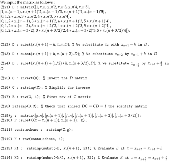
where I is the six by six identity matrix. We use the following wxMaxima(maple) codes to invert the D matrix as shown in the Appendix.

We are only interested in the first row of the C matrix which are,

c 11 = ( 24 x n + 1 5 + 15 h x n + 1 4 40 h 2 x n + 1 3 30 h 3 x n + 1 2 ) 31 h 5

c 12 = 24 x n + 1 5 + 15 h x n + 1 4 40 h 2 x n + 1 3 30 h 3 x n + 1 2 + 31 h 5 31 h 5

c 13 = ( 96 x n + 1 5 + 91 h x n + 1 4 98 h 2 x n + 1 3 89 h 3 x n + 1 2 ) 372 h 4

c 14 = ( 28 x n + 1 5 + 2 h x n + 1 4 57 h 2 x n + 1 3 4 h 3 x n + 1 2 + 31 h 4 x n + 1 ) 31 h 4

c 15 = ( 16 x n + 1 5 21 h x n + 1 4 6 h 2 x n + 1 3 + 11 h 3 x n + 1 2 ) 124 h 4

c 16 = 48 x n + 1 5 32 h x n + 1 4 80 h 2 x n + 1 3 + 64 h 3 x n + 1 2 93 h 4 .

Hence, we obtained the continuous coefficients

α 0 ( x ) = 24 ω 5 15 h ω 4 + 40 h 2 ω 3 + 30 h 3 ω 2 31 h 5

α 1 ( x ) = 24 ω 5 + 15 h ω 4 40 h 2 ω 3 30 h 3 ω 2 + 31 h 5 31 h 5

h β 0 ( x ) = 96 ω 5 91 h ω 4 + 98 h 2 ω 3 + 89 h 3 ω 2 372 h 4

h β 1 ( x ) = 28 ω 5 2 h ω 4 + 57 h 2 ω 3 + 4 h 3 ω 2 31 h 4 ω 31 h 4

h β 2 ( x ) = 16 ω 5 + 21 h ω 4 + 6 h 2 ω 3 11 h 3 ω 2 124 h 4

h β 3 2 ( x ) = 48 ω 5 32 h ω 4 80 h 2 ω 3 + 64 h 3 ω 2 93 h 4 .

If we substitute the above into (7), then we obtain the continuous scheme

y ¯ ( x ) = [ 24 ω 5 15 h ω 4 + 40 h 2 ω 3 + 30 h 3 ω 2 31 h 5 ] y n + [ 24 ω 5 + 15 h ω 4 40 h 2 ω 3 30 h 3 ω 2 + 31 h 5 31 h 5 ] y n + 1 + [ 96 ω 5 91 h ω 4 + 98 h 2 ω 3 + 89 h 3 ω 2 372 h 4 ] f n + [ 28 ω 5 2 h ω 4 + 57 h 2 ω 3 + 4 h 3 ω 2 31 h 4 ω 31 h 4 ] f n + 1 + [ 16 ω 5 + 21 h ω 4 + 6 h 2 ω 3 11 h 3 ω 2 124 h 4 ] f n + 2 + [ 48 ω 5 32 h ω 4 80 h 2 ω 3 + 64 h 3 ω 2 93 h 4 ] f n + 3 2 . (10)

We evaluated (10) at ω = h , ω = h 2 , ω = 3 h 4 and its derivative at ω = 3 h 4 .

We obtained the following four discrete schemes which constitutes the block method

y n + 2 = 1 31 y n + 32 31 y n + 1 + h 93 [ f n + 12 f n + 1 + 64 f n + 3 2 + 15 f n + 2 ] y n + 3 2 = 37 496 y n + 459 496 y n + 1 + h 1984 [ 39 f n + 648 f n + 1 + 480 f n + 3 2 27 f n + 2 ] y n + 7 4 = 243 7936 y n + 7693 7936 y n + 1 + h 31744 [ 231 f n + 7644 f n + 1 + 16464 f n + 3 2 + 441 f n + 2 ]

315 992 y n + 1 = 315 992 y n + h 1984 [ 179 f n 1169 f n + 1 + 2156 f n + 3 2 1984 f n + 7 4 + 546 f n + 2 ] . (11)

2.2. Convergence Analysis

We examine the order, error constant, zero stability and convergence of the discrete schemes in this paper.

α 0 = [ 1 31 37 496 243 7936 315 992 ] , α 1 = [ 32 31 459 496 7693 7936 315 992 ] , α 3 2 = [ 0 1 0 0 ] , α 7 4 = [ 0 0 1 0 ] , α 2 = [ 1 0 0 0 ] ,

and

β 0 = [ 1 93 39 1984 231 31744 179 1984 ] , β 1 = [ 12 93 648 1984 7644 31744 1169 1984 ] , β 3 2 = [ 64 93 480 1984 16464 31744 2156 1984 ] , β 7 4 = [ 0 0 0 1 ] , β 2 = [ 15 93 27 1984 441 31744 546 1984 ] .

Lemma 2.1: The order of each of the discrete schemes in the Two-Step Butchers scheme in block form (11) is uniformly 5.

Proof: In finding the order and error constant of the block scheme, we substituted the above vectors in the following formula.

C 0 = α 0 + α 1 + α 3 2 + α 7 4 + α 2 = 0

C 1 = [ α 1 + 2 α 2 + ( 3 2 ) α 3 2 + ( 7 4 ) α 7 4 ] [ β 0 + β 1 + β 2 + β 3 2 + β 7 4 ] = 0

C 2 = ( 1 2 ! ) [ α 1 + 2 2 α 2 + ( 3 2 ) 2 α 3 2 + ( 7 4 ) 2 α 7 4 ] [ β 1 + 2 β 2 + ( 3 2 ) β 3 2 + ( 7 4 ) β 7 4 ] = 0

C 3 = ( 1 3 ! ) [ α 1 + 2 3 α 2 + ( 3 2 ) 3 α 3 2 + ( 7 4 ) 3 α 7 4 ] ( 1 2 ! ) [ β 1 + 2 2 b 2 + ( 3 2 ) 2 β 3 2 + ( 7 4 ) 2 β 7 4 ] = 0

C 4 = ( 1 4 ! ) [ α 1 + 2 4 α 2 + ( 3 2 ) 4 α 3 2 + ( 7 4 ) 4 α 7 4 ] ( 1 3 ! ) [ β 1 + 2 3 β 2 + ( 3 2 ) 3 β 3 2 + ( 7 4 ) 3 β 7 4 ] = 0

C 5 = ( 1 5 ! ) [ α 1 + 2 5 α 2 + ( 3 2 ) 5 α 3 2 + ( 7 4 ) 5 α 7 4 ] ( 1 4 ! ) [ β 1 + 2 4 β 2 + ( 3 2 ) 4 β 3 2 + ( 7 4 ) 4 β 7 4 ] = 0

C 6 = ( 1 6 ! ) [ α 1 + 2 6 α 2 + ( 3 2 ) 6 α 3 2 + ( 7 4 ) 6 α 7 4 ] ( 1 5 ! ) [ β 1 + 2 5 β 2 + ( 3 2 ) 5 β 3 2 + ( 7 4 ) 5 β 7 4 ] = [ 1 5580 21 158720 147 10158080 231 253952 ]

The above formula showed that C 0 = C 1 = C 2 = C 3 = C 4 = C 5 = 0 and

Error Constant = [ 1 5580 21 158720 147 10158080 231 253952 ] 0 .

This implies that the order of each of the discrete schemes in the Two-step Butcher’s scheme in block form is 5.

The block method (11) can be represented as

[ 32 31 0 0 1 459 496 1 0 0 7693 7936 0 1 0 315 992 0 0 0 ] [ y n + 1 y n + 3 / 2 y n + 7 / 4 y n + 2 ] = [ 1 0 0 0 0 1 0 0 0 0 1 0 0 0 0 1 ] [ y n 2 y n 3 / 2 y n 1 y n ] + h [ 1 93 4 31 64 93 0 5 31 39 1984 81 248 15 62 0 27 1984 231 31744 1911 7936 1029 1984 0 441 31744 179 1984 1169 1984 539 496 1 273 992 ] [ f n + 1 f n + 3 / 2 f n + 7 / 4 f n + 2 ] + h [ 0 0 0 1 93 0 0 0 39 1984 0 0 0 231 31744 0 0 0 179 1984 ] [ f n 3 f n 2 f n 1 f n ] .

In addition, we need the following matrices in analysing the zero stability of the block method,

A ( 0 ) = [ 32 31 0 0 1 459 496 1 0 0 7693 7936 0 1 0 315 992 0 0 0 ] , and B ( 0 ) = [ 0 0 0 1 31 0 0 0 37 496 0 0 0 243 7936 0 0 0 315 992 ] .

The characteristic polynomial corresponding to (11) is given as

ρ ( R ) = det ( R A ( 0 ) B ( 0 ) ) = | 32 31 R 0 0 R 1 31 459 496 R R 0 37 496 7693 7936 R 0 R 243 7936 315 992 R 0 0 315 992 | = 315 R 4 + 315 R 3 992 = 0.

The roots of the characteristic equation ρ ( R ) = R 4 + R 3 = R 3 ( R + 1 ) = 0 are R = 0 (thrice) and R = 1 . This leads to the following result.

Lemma 2.2: The Two-step Butchers scheme in block form (11) is zero stable, consistent and hence convergent.

Proof: By definition, a Linear Multistep Method is said to be zero-stable if none of the roots of its characteristic polynomial has modulus greater than one and each of the roots with modulus one must be distinct. This is immediate from above. As shown in Lemma 2.1 the order of the Two-step scheme is p = 5 which is greater than one. Therefore, consistency is established [21]. Since it is both zero-stable and consistent, by definition, it is convergent.

2.3. Region of Absolute Stability

To plot the region of absolute stability of the Two-step Butcher’s scheme we used the following stability matrix equation

M ( z ) = C + z B ( I z A ) 1 D ,

then we substituted it into the stability polynomial in line with Chollom [3]

ρ ( r , z ) = det ( r I M ( z ) ) ,

where I is the identity matrix of size M ( z ) . We then used Newton’s method in finding the roots of the stability polynomial and plotted the resultant roots where the region of absolute stability of the method is defined as

E ( z ) = { z : ρ ( r , z ) = 1 , | r | 1 } .

The region of absolute stability of the Two-Step Butcher’s scheme is as shown in Figure 1. We obtained the matrices A , B , C and D from the discrete schemes in this fashion:

Figure 1. Region of absolute stability of the Two-Step Butcher’s scheme.

[ y n y n + 1 y n + 3 / 2 y n + 7 / 4 y n + 2 y n + 2 y n + 1 y n ] = [ A D B C ] [ h f n h f n + 1 h f n + 3 / 2 h f n + 7 / 4 h f n + 2 y n + 2 y n + 1 y n ] ,

where the matrices are respectively

A = [ 0 0 0 0 0 1 93 4 31 64 93 0 5 31 39 1984 81 248 15 62 0 27 1984 231 31744 1911 7936 1029 1984 0 441 31744 179 1984 1169 1984 539 496 1 273 992 ] ,

B = [ 179 1984 1169 1984 539 496 1 273 992 1 93 4 31 64 93 0 5 31 0 0 0 0 0 ] ,

C = [ 0 315 992 315 992 1 1 31 1 31 0 0 1 ] ,

and

D = [ 0 0 1 1 32 31 1 31 0 459 496 37 496 0 7693 7936 243 7936 0 315 992 315 992 ] .

So far, we have discussed in great detail the Two-step Butcher’s hybrid scheme in block form. The 5th order Butcher’s algorithm in Lambert [19] consists of three sets of equations, the first two are used as predictors while the last (Two-step Butcher’s scheme) is used as a corrector. In a nutshell, the 5th order algorithm is as follows

y n + 3 / 2 y n = h 8 [ 9 f n + 1 + 3 f n ] ( Predictor ) y n + 2 1 5 ( 28 y n + 1 23 y n ) = 2 h 15 [ 30 f n + 1 13 f n + 16 f n + 3 / 2 ] ( Predictor ) y n + 2 + 1 31 y n + 32 31 y n + 1 = h 93 [ f n + 12 f n + 1 + 64 f n + 3 2 + 15 f n + 2 ] ( Corrector ) (12)

It is not self starting unlike the former relying on good initial guesses. Now, notice that

α 0 = [ 1 23 5 ] , α 1 = [ 0 28 5 ] , α 3 2 = [ 1 0 ] , α 2 = [ 0 1 ] ,

and

β 0 = [ 3 8 26 15 ] , β 1 = [ 9 8 4 ] , β 3 2 = [ 0 0 ] , β 2 = [ 0 32 15 ] .

Lemma 2.3: The order of each of the discrete schemes (predictors) in the 5th order Butchers algorithm in block form (12) is 3.

Proof: In finding the order and error constant of the block scheme, we substituted the above vectors in the following formula.

C 0 = α 0 + α 1 + α 3 2 + α 2 = 0

C 1 = [ α 1 + 2 α 2 + ( 3 2 ) α 3 2 ] [ β 0 + β 1 + β 2 + β 3 2 ] = 0

C 2 = ( 1 2 ! ) [ α 1 + 2 2 α 2 + ( 3 2 ) 2 α 3 2 ] [ β 1 + 2 β 2 + ( 3 2 ) β 3 2 ] = 0

C 3 = ( 1 3 ! ) [ α 1 + 2 3 α 2 + ( 3 2 ) 3 α 3 2 ] ( 1 2 ! ) [ β 1 + 2 2 β 2 + ( 3 2 ) 2 β 3 2 ] = 0

C 4 = ( 1 4 ! ) [ α 1 + 2 4 α 2 + ( 3 2 ) 4 α 3 2 ] ( 1 3 ! ) [ β 1 + 2 3 β 2 + ( 3 2 ) 3 β 3 2 ] = [ 3 128 1 10 ]

The above formula showed that C 0 = C 1 = C 2 = C 3 = 0 and

Error Constant = [ 3 128 1 10 ] 0 .

This implies that the order of each of the discrete schemes in the Two-step Butcher’s scheme in block form is 3.

3. Numerical Experiments

In this section, we applied both the derived discrete scheme in block form and the schemes given in Lambert [19] in Predictor-Corrector form on some initial value problems.

Example 3.1

Consider the following initial value problem y = y with initial condition y ( 0 ) = y 0 = 1 , h = 0.2 on 0 x 2.4 and y ( x ) = e x as exact solution.

Using the above Two-Step Butcher’s scheme in block form with y = f ( x , y ) = y . In matrix form for n = 0 , (11) becomes respectively,

[ 240 234 0 32 27 8532 0 10400 441 146216 158720 16464 546 4319 1984 2156 ] [ y 1 y 3 2 y 7 4 y 2 ] = [ 7 701 4629 2971 ] . (13)

For n = 2 , we have the same matrix as above but different right hand side

[ 240 234 0 32 27 8532 0 10400 441 146216 158720 16464 546 4319 1984 2156 ] [ y 3 y 7 2 y 15 4 y 4 ] = [ 7 701 4629 2971 ] y 2 = [ 4.692239 469.894282 3102.911030 1991.520559 ] . (14)

This process is continued for n = 4 , 6 , 8 , , 30 and the results are as shown in Figures 2-5. It can be observed from the first four figures of Figure 2 that the Two-Step Butcher’s scheme in block form performed at par with the exact solution. Since we are solving a linear system of equations in each iteration, we plotted the values of n against the norm of the residual r = b A y on a semilogy

Figure 2. Comparison of the approximate values of y n + 1 , y n + 3 / 2 , y n + 7 / 4 , y n + 2 obtained using the Two-Step Butcher’s scheme and the exact solution.

Figure 3. The norm of the residual r = b A y versus the values of n on a semilogy scale obtained from using the Two-Step Butcher’s scheme.

Figure 4. The norm of the error between exact and approximate y n using the Two-Step Butcher’s scheme in block form.

Figure 5. Absolute errors of the 5th Order Butcher’s algorithm with y 1 the same obtained from the Two-Step Butcher’s Scheme.

scale and the result is as shown in Figure 3. It can be observed that as n increases, the norm of the residual decreases as expected. In the same vein, Figure 4 shows a plot of the norm of the Error between the Exact and Approximate values of y n using the Two-Step Butcher’s scheme in block form on a semilogy scale.

In addition, we used the 5th Order Butcher’s algorithm to solve the same initial problem. Since this algorithm is non self starting, we made two different plots shown by the red and blue lines of Figure 5 and Figure 6. In Figure 5, we used the exact value of y 1 as starting guess in solving the IVP, while in Figure 6, we used the y 1 obtained from the Two-Step Butcher’s scheme in solving the IVP and the absolute errors are plotted on semilogy scales. We observed that except for n = 0 , 1 , 2 , 3 , 4 , 5 , there is no distinctive difference between the two red and blue plots in both figures. In the aforementioned figures, we also super-imposed the solution obtained from an implementation of the Two-Step Butcher’s scheme on the same figures for better comparison. These are clearly shown by the lower yellow and black lines depicting better approximate solutions. Since the 5th Order Butcher’s algorithm uses the exact value of y 1 , one would have expected that it will give better approximations to the exact solution. However, for both y n + 3 / 2 and y n + 2 , the Two-Step Butcher’s scheme in block form outperformed the former. Besides, in the absence of round off errors while it took the Two-Step Butcher’s scheme n = 30 (=2(30)) iterations, it took the 5th Order Butcher’s scheme n = 60 iterations.

Figure 6. Absolute errors of the 5th Order Butcher’s algorithm with y 1 as exact value against Number of iterations.

Example 3.2

Consider the following initial value problem y = 20 y + 20 sin x + cos x with initial condition y ( 0 ) = y 0 = 1 , h = 0.1 on 0 x 3.2 . Using the Two-Step Butcher’s scheme in block form we substitute f ( x , y ) = 20 y + 20 sin x + cos x and for n = 0 , we obtained the following system of equations

[ 170 1280 0 1230 5400 29440 0 540 154840 32980 317440 8820 29680 43120 39680 10920 ] [ y 1 y 3 2 y 7 4 y 2 ] = [ 353.7640264 4453.076732 95869.93272 3978.425343 ] . (15)

For n = 2 , we obtained the following system of equations

[ 170 1280 0 1230 5400 29440 0 540 154840 32980 317440 8820 29680 43120 39680 10920 ] [ y 3 y 7 2 y 15 4 y 4 ] = [ 10 700 5100 2720 ] y 2 + [ 1022.257690852725 12221.5143372693 273505.2293709757 6045.327476872326 ] .

This process is continued for n = 4 , 6 , 8 , , 30 and the results are as shown in Figures 7-10. It can be observed from the first four figures of Figure 7 that the Two-Step Butcher’s scheme in block form performed at par with the exact solution. In addition, Figure 8 shows a plot of computed absolute errors of y n + 1 , y n + 3 / 2 , y n + 7 / 4 , y n + 2 using the Two-Step Butcher’s scheme in block form. The black line showed that y n + 2 had the least absolute error compared to the rest. Since we are solving a linear system of equations in each iteration, we plotted the values of n against the norm of the residual r = b A y on a semilogy scale and the result is as shown in Figure 9. We observed that as n increases, the norm of the residual decreases as expected. In the same vein, Figure 10 shows a plot of the norm of the Error between the Exact and Approximate values of y n using the Two-Step Butcher’s scheme in block form on a semilogy scale. However, unlike the first example in which the 5th Order Butcher’s algorithm performed well, here we noticed a great divergence from the exact values. This means that this algorithm is not suitable for problems of this nature albeit the trigonometric functions involved. This shows the supremacy of the Two-Step Butcher’s scheme for solving IVPs.

Example 3.3

We seek numerical approximations to the initial value problem y = 9 y with initial condition y ( 0 ) = e , h = 0.1 .

We followed the same steps in solving Examples 3.1 and 3.2. We started with n = 2 , this process was continued for n = 4 , 6 , 8 , , 30 and the results are as

Figure 7. Comparison of the approximate values of y n + 1 , y n + 3 / 2 , y n + 7 / 4 , y n + 2 obtained using the Two-Step Butcher’s scheme and the exact solution.

Figure 8. Absolute errors of y n + 1 , y n + 3 / 2 , y n + 7 / 4 , y n + 2 using the Two-Step Butcher’s scheme in block form.

Figure 9. The norm of the residual r = b A y versus the values of n on a semilogy scale obtained from using the Two-Step Butcher’s scheme.

Figure 10. The norm of the error between the exact and approximate values of y n using the Two-Step Butcher’s scheme in block form versus the number of iterations.

shown in Figures 11-15. It can be observed from the first four figures of Figure 11 that the Two-Step Butcher’s scheme in block form performed at par with the exact solution. Since we are solving a linear system of equations in each iteration, we plotted the values of n against the norm of the residual r = b A y on a semilogy scale and the result is as shown in Figure 12. It can be observed that as n increases, the norm of the residual decreases as expected. In the same vein, Figure 13 shows a plot of the norm of the Error between the Exact and Approximate values of y n using the Two-Step Butcher’s scheme in block form on a semilogy scale.

In addition, we used the 5th Order Butcher’s algorithm to solve the same initial problem. Since this algorithm is non self starting, we made two different plots shown by the red and blue lines of Figure 14 and Figure 15. In Figure 14, we used the exact value of y 1 as starting guess in solving the IVP, while in Figure 15, we used the y 1 obtained from the Two-Step Butcher’s scheme and the absolute errors are plotted on semilogy scales. We observed that except for

n = 0 , 1 , 2 , 3 , 4 , 5 , there is no distinctive difference between the two red and blue plots in both figures. In the aforementioned figures, we also super-imposed the solution obtained from an implementation of the Two-Step Butcher’s scheme on the same figures for better comparison. These are clearly shown by the lower yellow and black lines depicting better approximate solutions. For example, at

Figure 11. Comparison of the approximate values of y n + 1 , y n + 3 / 2 , y n + 7 / 4 , y n + 2 obtained using the Two-Step Butcher’s scheme and the exact solution.

Figure 12. The norm of the residual r = b A y versus the values of n on a semilogy scale obtained from using the Two-Step Butcher’s scheme.

Figure 13. The norm of the error between exact and approximate y n using the Two-Step Butcher’s scheme in block form.

Figure 14. Absolute errors of the 5th Order Butcher’s algorithm with y 1 the same obtained from the Two-Step Butcher’s Scheme.

Figure 15. Absolute errors of the 5th Order Butcher’s algorithm with y 1 as exact value against Number of iterations.

n = 30 in Figure 14 and Figure 15, while the minimum absolute error obtained using the Two-Step Butcher’s scheme is approximately 10−25, that of the 5th Order Butcher’s algorithm is approximately 10−10 of course in the absence of round off errors. Since the 5th Order Butcher’s algorithm uses the exact value of y 1 , one would have expected that it will give better approximations to the exact solution. However, for both y n + 3 / 2 and y n + 2 , the Two-Step Butcher’s scheme in block form outperformed the former.

4. Conclusion

We showed that if the step size h is not too small the matrix D will be invertible. Nowhere in literature has there been any proof on the necessary conditions for the invertibility of the D matrix which was our main aim. In addition, ordinarily speaking one would have expected the 5th Order Butcher’s algorithm which uses the exact solution y 1 as the starting value to give more accurate results than the self-starting Two-step Butcher’s scheme in block form, but to our greatest surprise, the reverse was the case as depicted by the Figureof the absolute errors in the preceding section. The accuracy could be due to the fact that all the discrete schemes used in the Two-step Butcher’s scheme in block form are of uniform order. From the figures in the last section, we can confidently say that the Two-step Butcher’s hybrid scheme performed better than its counterpart. In addition, the former performs well for both stiff and non-stiff IVPs.

Acknowledgements

The effort of Prof. U. W. W. Sirisena, who guided the first author’s project, is acknowledged.

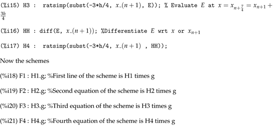
Appendix. wxMaxima Codes for the Analysis

NOTES

1We used brute force in doing so in [2], but here we show the Maxima codes for doing so.

Conflicts of Interest

Authors have declared that no competing interests exist.

References

[1] Sirisina, U.W., Kumleng, G.M. and Yahaya, Y.A. (2004) A New Butcher Type Two-Step Block Hybrid Multistep Method for Accurate and Efficient Parallel Solution of Ordinary Differential Equations. Abacus Mathematics Series, 31, 1-7.
[2] Akinola, R.O. (2001) An Accurate Implementation of the Two-Step Butcher’s Hybrid Scheme on Initial Value Problems. BSc Thesis, University of Jos, Jos.
[3] Chollom, J.P., Ndam, J.N. and Kumleng, G.M. (2007). On Some Properties of the Block Linear Multistep Methods. Science World Journal, 2, 11-17.
https://doi.org/10.4314/swj.v2i3.51747
[4] Maxima 5.42.1. (n.d.)
https://maxima.sourceforge.io/
[5] Maplesoft, a Division of Waterloo Maple Inc. (2019). Maple. Waterloo, Ontario.
[6] Eaton, J.W., Bateman, D., Hauberg, S. and Wehbring, R. (2018) GNU Octave Version 4.4.1 Manual: A High-Level Interactive Language for Numerical Computations.
[7] The MathWorks Inc. (2019) MATLAB. 9.7.0.1190202. Natick.
[8] Chollom, J.P., Olatunbosun, I.O. and Omagu, S. (2012) A Class of A-Stable Block Explicit Methods for the Solutions of ODEs Research. Journal of Mathematics and Statistics, 4, 52-56.
[9] Kumleng, G.M. and Skwame, Y. (2011) A New A-Stable Method for the Solution of Stiff Initial Value Problems. International Journal of Numerical Maths, 6, 360-373.
[10] Kumleng, G.M., Sirisena, U.W. and Chollom, J.P. (2012) Construction of a Class of Block Hybrid Implicit Multistep Methods for the Solution of Stiff Ordinary Differential Equations. Nigerian Journal of Pure and Applied Sciences, 5.
[11] Kumleng, G.M, Longwap, S. and Adee, S.O. (2013) A Class of A-Stable Order Four and Six Linear Multistep Methods for Stiff Initial Value Problems. Mathematical Theory and Modeling, 3, 1-10.
[12] Kamoh, N.M., Aboiyar, T. and Onah E.S (2017) On One Investigating Some Quadrature Rules for the Solution of Second Order Volterra Integro-Differential Equations. IOSR Journal of Mathematics (IOSR-JM), 13, 45-50.
[13] Yahaya, Y.A. and Badmus A.M. (2010) A Class of Collocation Methods for General Second Order Ordinary Differential Equations. African Journal of Mathematics and Computer Science Research, 2, 69-72.
[14] Yahaya, Y.A. and Adegboye Z.A. (2012) Construction and Implementation of a 4-Step Implicit Collocation Method for Solution of First and Second Order ODEs. Pacific Journal of Science and Technology, 13, 159-165.
[15] Kamoh, N.M., Gyemang, D.G. and Soomiyol, M.C. (2017) On One Justification on the Use of Hybrids for the Solution of First Order Initial Value Problems of Ordinary Differential Equations. Pure and Applied Mathematics Journal, 6, 137-143.
https://doi.org/10.11648/j.pamj.20170605.11
[16] Kumleng, G.M. and Sirisena, U.W.W. (2014) A (α)-Stable Order Ten Second Derivative Block Multistep Method for Stiff Initial Value Problems. International Journal of Mathematics and Statistics Invention (IJMSI), 2, 37-43.
[17] Bakari, A., Skwame, I.Y. and Kumleng, G.M. (2018) An Application of Second Derivative Backward Differentiation Formula Hybrid Block Method on Stiff Ordinary Differential Equations. Journal of Natural Sciences Research, 8, 27-36.
[18] Scheffel, J. and Lindvall, K. (2018) Optimizing Time-Spectral Solution of Initial-Value Problems. American Journal of Computational Mathematics, 8, 7-26.
https://doi.org/10.4236/ajcm.2018.81002
[19] Lambert, J.D. (1973) Computational Methods in Ordinary Differential Equations. John Wiley & Sons, New York.
[20] Onumanyi, P., Awoyemi, D.O., Jator, S.N. and Sirisena, U.W. (1994) New Linear Multistep Methods with Continuous Coefficients for First Order Initial Value Problems. Journal of Nigeria Mathematics Society, 13, 37-51.
[21] Henrici, P. (1962) Discrete Variable Methods in Ordinary Differential Equations. Wiley, New York, 407 p.

Copyright © 2024 by authors and Scientific Research Publishing Inc.

Creative Commons License

This work and the related PDF file are licensed under a Creative Commons Attribution 4.0 International License.