A Theoretical Comparison among Recursive Algorithms for Fast Computation of Zernike Moments Using the Concept of Time Complexity

Nasrin Bastani^1,2,3*, Alireza Vard^1,2, Mehdi Jabalameli³, Vahid Bastani⁴

¹School of Advanced Technologies in Medicine, Isfahan University of Medical Sciences, Isfahan, Iran.
²Medical Image and Signal Processing Research Center, Isfahan University of Medical Sciences, Isfahan, Iran.
³Computer Department, Islamic Azad University Najafabad Branch, Isfahan, Iran.
⁴English Department, Islamic Azad University Najafabad Branch, Isfahan, Iran.

DOI: 10.4236/ajcm.2021.114020                

Abstract

Zernike polynomials have been used in different fields such as optics, astronomy, and digital image analysis for many years. To form these polynomials, Zernike moments are essential to be determined. One of the main issues in realizing the moments is using factorial terms in their equation which causes higher time complexity. As a solution, several methods have been presented to reduce the time complexity of these polynomials in recent years. The purpose of this research is to study several methods among the most popular recursive methods for fast Zernike computation and compare them together by a global theoretical evaluation system called worst-case time complexity. In this study, we have analyzed the selected algorithms and calculated the worst-case time complexity for each one. After that, the results are represented and explained and finally, a conclusion has been made by comparing these criteria among the studied algorithms. According to time complexity, we have observed that although some algorithms such as Wee method and Modified Prata method were successful in having the smaller time complexities, some other approaches did not make any significant difference compared to the classical algorithm.

Keywords

Time Complexity, Uniform Model, Zernike Moments, Zernike Polynomi-als

1. Introduction

Zernike polynomials are widely used in different fields such as optics, astronomy science and digital image analysis. They are able to describe every circular aperture since they have orthogonality over this type of aperture [1]. They could be used in wavefront reconstruction applications [2], object-class detection [3] [4] [5] [6], image classification [7], feature extraction [8] [9], brain tumor diagnosis [10], or even cone dimensions detection in keratoconus [11].

Zernike polynomials have a mathematical definition for optical aberration [12]. These polynomials have been used for more than seventy years in optical applications [13]. Moreover, they are able to describe both fixed and random aberrations [14] and model optical surfaces such as telescope mirrors or corneal topography [15]. Zernike polynomials are able to determine the primary shape of the optical surface and remove individual terms with no effect on the value of reminded terms [16].

Many of the applications that use Zernike polynomials, are related to eye aberration [17]. Eye aberration is the distortion of human vision and is measured using the reflected wavefront at pupil [18]. The wavefront is expressed by measured gradients related to each reflected point [19] and various types of abnormality are classified by Zernike polynomial set [20]. As a result, to form these polynomials, Zernike moments are essential to be determined. These moments are defined as the projection of 1D (speech)/2D (image) signals onto Zernike polynomials. One of the main issues in computing the moments is using factorial terms. Factorial terms cause a heavy computational load and a large time complexity. Therefore, this problem makes Zernike polynomials less proper to be used in real time applications.

In this paper, we have studied the most popular recursive algorithms which tried to reduce the time complexity of Zernike moments [21] - [27]. We have assessed and compared their efficiency by computing the worst-case time complexity.

The paper is organized as follows: we have described the primary concepts related to the time complexity in the next Section. In Section 3, we have introduced Zernike polynomials, Zernike moments, and the classical approach to obtain the moments. Section 4 is specified to some of the popular algorithms that have been existed to decrease the time complexity of Zernike moments, and comparative results and discussion are available in Section 5. Finally, we have the conclusion in Section 6.

2. Primary Concepts of Time Complexity

Time complexity is a criterion to evaluate algorithms. This concept is defined as the minimum time resource that the algorithm needs to be completed considering all of the exceptional situations. Time complexity is classified to theoretical time complexity and practical time complexity. The second, known as running time, is only available on code lines and applications. In addition, this concept is completely dependent on the machine while theoretical time complexity is an absolute independent estimation [28]. Consequently, practical time complexity is an unreliable criterion since different computers have different hardware properties; on the contrary, theoretical time complexity is a global independent standard to evaluate time efficiency of an algorithm [29]. To clarify this matter, the definitions of the two concepts are provided.

Running time of program A is the number of moves A makes (on input x) until the program is completed [30]. The moves are in either time unit or instruction unit. In other words, to calculate the running time of a program we should count the instructions or measure the time until the program completes its function. Numbering instructions of a program is not a standard method to evaluate time efficiency since there are differences between programming languages that the algorithm is implemented by [29]. In addition, the number of instruction lines may differ depending on the programmer choices. Measuring the time unit is not a reliable evaluation because hardware features may vary in different computers [29].

While running time is totally dependent on the program, theoretical time complexity is the number of statements executed by the algorithm on input x [31]. It is based on the raw algorithm and counts the number of the main operation until the algorithm halts [29]. Theoretical time complexity may be evaluated by the exact case, the best case, the average case, or the worst case analysis functions.

The best case time complexity, the average case time complexity, and the worst case time complexity are detected by the minimum, the average, or the worst repetition rate of the main operation respectively and the final result is a function of the size of the input string.

The worst case analysis function has been widely used to estimate time efficiency of an algorithm. The standard notation for this assessment is Big-Oh (O) notation [32]. It ignores worthless details in calculations and determines the certain time bound in which an algorithm can be completed [32] [33]. As a mathematical expression, the exact time complexity $f\left(n\right)$ is of $O\left(g\left(n\right)\right)$ if there are positive constants such C and k (k is integer) that for all input string length $n>k$, $f\left(n\right)\le C\cdot g\left(n\right)$ [34]. This situation is addressed as $f\left(n\right)$ is Big-Oh of $g\left(n\right)$.

Figure 1 shows the difference between the exact time complexity and the worst case time complexity, represented by a black line and a blue line respectively. As we can observe, if the exact time complexity of an algorithm

equals $0.723\ast 3^x+{1.618}^{\frac{x}{2}}$, the related worst case time complexity will be $3^x$.

The other subject to discuss is the model of the calculations. Generally, there are two models to calculate theoretical time complexity [35]. A uniform model supposes that all operations on any size of input take the same constant time to be completed while a non-uniform model allocates a unique computation time to each operation that is executed on every single input length [35]. Uniform models are common for algorithms with low domain numbers while a non-uniform model is recommended to evaluate the algorithms that have large length inputs.

Figure 1. An example of the exact time complexity and the worst-case time complexity.

In this study, we use the uniform model and the worst-case time complexity to evaluate time efficiency of the selected algorithms. The worst-case time complexity has been chosen since this assessment delivers us the maximum time unit taken by the algorithm. The uniform model has been selected due to low domain size of input strings used in Zernike moments. The input string is the order of the polynomial and doesn’t go further than 15 in the researches [36]. In fact, the notable information is represented by moments up to order 15 [37]. This number doesn’t take a considerable time complexity in computational operations and as a result, using uniform model is completely acceptable for this purpose.

3. Classical Method to Calculate Zernike Moments

Zernike polynomials have been introduced by Frits Zernike in 1934 [38]. They are featured by having orthogonality in a continuous circle with unit radius [39] and are able to describe every function of wavefront aberration or phase [1].

In a discontinuous environment, Zernike polynomials model wavefront representation [1] [40] [41] using (1),

$W\left(\rho ,\theta \right)={\displaystyle \underset{n=1}{\overset{N}{\sum }}}{\displaystyle \underset{m=0}{\overset{n}{\sum }}}{C}_n^m{Z}_n^m\left(\rho ,\theta \right)+\epsilon$ (1)

$C_n^m$ is Zernike moment in azimuthal frequency m and polynomial order n. The parameters $\rho \mathrm{,}\theta$ are the elements of the polar coordinate centered around the aperture. $\rho$ must be normalized as it is limited to unitary cycle. $\theta$ is the angle in polar coordinate, and $W\left(\rho ,\theta \right)$ is the reconstructed wavefront. N shows the maximum order that has been used to model the wavefront. The maximum value of N is 15 in researches [36] while in clinical diagnosis, calculations are up to forth order [42]. $\epsilon$ represents the error of modeling and measuring the wavefront. It is assumed that the input noise is idd random noise with a zero valued average and a constant variance [40] [43].

Radial normalization is calculated using (2),

$\rho =\frac{r}{r_{pup}}$ (2)

r is the distance between off-center and center points. $r_{pup}$ is the radius of aperture.

Radial function [1] [36] [39] [40] [43] is defined by (3),

$R_n^m\left(\rho \right)=\{\begin{array}{l}{\displaystyle {\sum }_{s=0}^{\frac{n-\left|m\right|}{2}}\frac{{\left(-1\right)}^s\left(n-s\right)!}{s!\left[0.5\left(n+\left|m\right|\right)-s\right]!\left[0.5\left(n-\left|m\right|\right)-s\right]!}}\left|m\right|\le n,n-m=\text{even}\\ 0\text{otherwise}\end{array}$ (3)

Finally, Zernike polynomials [1] [40] are determined using (4),

$z_n^m\left(\rho ,\theta \right)=\{\begin{array}{l}{N}_n^m{R}_n^m\left(\rho \right)\cos m\theta m\ge 0,0\le \rho \le 1,0\le \theta \le 2\pi \\ -N_n^m{R}_n^m\left(\rho \right)\sin m\theta m<0,0\le \rho \le 1,0\le \theta \le 2\pi \end{array}$ (4)

$N_n^m$ is the normalization factor defined [1] [40] as follows:

$N_n^m=\sqrt{\frac{2\left(n+1\right)}{1+{\delta }_{m0}}},$ (5)

${\delta }_{m0}$ is the regular delta function. We can merge (4) and (5) and rewrite Zernike polynomials [36] [39] [40] [44] as (6):

$z_n^m\left(\rho ,\theta \right)=\{\begin{array}{ll}\sqrt{2\left(n+1\right)}{R}_n^m\left(\rho \right)\cos \left(m\theta \right)\hfill & m>0,0\le \rho \le 1,0\le \theta \le 2\pi \hfill \\ \sqrt{2\left(n+1\right)}{R}_n^m\left(\rho \right)\sin \left(\left|m\right|\theta \right)\hfill & m<0,0\le \rho \le 1,0\le \theta \le 2\pi \hfill \\ \sqrt{2\left(n+1\right)}{R}_n^m\left(\rho \right)\hfill & m=0,0\le \rho \le 1,0\le \theta \le 2\pi \hfill \end{array}$ (6)

$c_n^m={\displaystyle {\int }_0^1}{\displaystyle {\int }_0^1}W\left(\rho \mathrm{,}\theta \right)Z_n^m\left(\rho \mathrm{,}\theta \right)\rho \text{d}\theta \text{d}\rho$ (7)

$C_n^m=\{\begin{array}{ll}{\displaystyle {\sum }_{\rho \le 1}{\displaystyle \sum W\left(\rho ,\theta \right)Z_n^m\left(\rho ,\theta \right)}}\hfill & m\ge 0\hfill \\ {\displaystyle {\sum }_{\rho \le 1}{\displaystyle \sum -W\left(\rho ,\theta \right)Z_n^m\left(\rho ,\theta \right)}}\hfill & m<0\hfill \end{array}$ (8)

After transformation to the discontinuous environment, Zernike moments are determined by (8) [1]. Negative values of m doubles the time complexity, however, it does not change the order. Consequently, we ignore negative values of this variable in the rest of the article.

To evaluate the time complexity of Zernike moments, we obtain the time complexity of radial functions at first. The main operation is different in every term of the expression (Table 1). Each term is repeated in a loop to construct the radial function. Table 2 represents the number of repetitions for each term and the related time complexity. The reason to consider multiplication as the main operation of factorial terms, and compare as the main operation of ${\left(-1\right)}^s$ could

Table 1. Time complexity of each term in the equation of radial function for 1 time.

Table 2. Number of repetitions for each term until the algorithm halts and the total time complexity related to the expression.

be discussed as following: To calculate $n!$, the below algorithm is used:

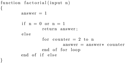
As we can observe, we have a compare operation to check if $n=0$ or $n=1$ which is the main operation in the case of $n=0$ or $n=1$. Then, if $n>1$ the loop will start and the multiple will be the main operation.

The other term is ${\left(-1\right)}^s$. The reason is that ${\left(-1\right)}^s$ could be implemented as below easily without any exceeded calculation:

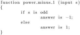
It only needs a comparison operation to realize the result.

To compute a complete set of radial functions, the equation needs

$m=\text{mode}\left(\frac{n}{2}\right)\mathrm{,}\text{mode}\left(\frac{n}{2}\right)+\mathrm{2,}\cdots \mathrm{,}n$, $n-m=\text{even}$. Then, we calculate the total

time complexity which is independent of m as follows:

$\begin{array}{l}T\left(n\right)={\displaystyle \underset{i=0}{\overset{\lfloor \frac{n}{2}\rfloor }{\sum }}}\frac{33n^2-26n\left(2i\right)+104n-7{\left(2i\right)}^2-8\left(2i\right)+64}{32}\\ =\frac{53n^3+399n^2+778n+384}{192}\Rightarrow \\ T\left(N\right)=\frac{53N^4+638N^3+2407N^2+3358N+1536}{768}\in O\left(N^4\right)\end{array}$ (9)

N is the maximum order used by the algorithm. To obtain the total time complexity for each n, we have added a summation expression to $T\left(m\mathrm{,}n\right)$.

Summation limitation is in $\left[\mathrm{0,}\frac{n}{2}\right]$ and we have replaced m with:

$m=2i+\text{mode}\left(\frac{n}{2}\right)\mathrm{,}i=\mathrm{0,1}\cdots \mathrm{,}\lfloor \frac{n}{2}\rfloor$ (10)

Then, we have used i instead of m. $\text{mode}\left(\frac{n}{2}\right)$ is the reminder when n is

devided by 2 which can be ignored.

Finally, a complete set of radial functions could be computed in $O\left(N^4\right)$ for each point of the image. According to (6), $Z_n^m\left(\rho \mathrm{,}\theta \right)$ has the same worst-case time complexity with $R_n^m\left(\rho \right)$. As a result, a complete set of Zernike polynomials has the worst-case time complexity of $O\left(M^2{N}^4\right)$ for a $M\times M$ image.

As we can observe, factorial terms and power terms would be obtained recursively by $n!=n\left(n-1\right)!$ and ${\rho }^s=\rho \times {\rho }^{s-1}$.

4. Fast Methods to Calculate Zernike Moments

In this section, we will study seven best known recursive methods that tried to reduce the time complexity of Zernike moments. We have selected recursive methods due to their success in this aim. In the following, we will consider these fast algorithms.

4.1. Kintner Method

In 1976, Kintner represented his method to calculate radial functions and used a pure recursive relationship with three terms [21]. This recursive function is represented by:

$K_1{R}_{n+2}^m\left(\rho \right)=\left(K_2{\rho }^2+K_3\right)R_n^m\left(\rho \right)+K_4{R}_{n-2}^m\left(\rho \right)$ (11)

And the coefficients $K_i,1\le i<4$ are defined using:

$\begin{array}{l}{K}_1=2n\left(\frac{n+m}{2}+1\right)\left(\frac{n-m}{2}+1\right)\\ K_2=2n\left(n+1\right)\left(n+2\right)\\ K_3=-m^2\left(n+1\right)-n\left(n+1\right)\left(n+2\right)\\ K_4=-2\left(\frac{n+m}{2}\right)\left(\frac{n-m}{2}\right)\left(n+2\right)\end{array}$ (12)

$R_{m+2}^m$ and $R_m^m$ are calculated through the classical method.

To start with the coefficients, multiplication is the main operation. $K_1\mathrm{,}{K}_2\mathrm{,}{K}_3\mathrm{,}{K}_4$ need 5, 3, 5, 6 multiplications respectively. Devision, expontiation, and multiplying by −1 are considered as multiplication as well. Each $R_n^m\left(\rho \right)$ has 6 multiplications in its equation. As a result, to calculate the time complexity of $R_n^m\left(\rho \right)$, we need 25 multiplications. As we can see in Figure 2, $R_n^m\left(\rho \right)$ could be ontained when $R_{n-2}^m\left(\rho \right)$ and $R_{n-4}^m\left(\rho \right)$ are determined. Thus we can obtain $T\left(m\mathrm{,}n\right)$ by (13)

$T\left(n,m\right)=25+T\left(m,n-2\right)+T\left(m,n-4\right)$ (13)

If we sketch the binary tree of the time complexity (Figure 2), it is obvious that there is 2⁰ node in the first level, 2¹ nodes in the second layer, 2² nodes in the third layer, and in general $2^{n-m-4}$ nodes in the layer before the last layer. Thus,

Figure 2. Kintner method, the binary tree of the time complexity, top-down programming.

we have ${\displaystyle {\sum }_{i=0}^{n-m-4}}{2}^i$ nodes. Each node needs 25 multiplications. Therefore, we have $T\left(m\mathrm{,}n\right)$ by (14):

$T\left(m,n\right)={\displaystyle \underset{j=0}{\overset{n-m-4}{\sum }}}25\times 2^j=25\times \left[2^{n-m-3}-1\right]$ (14)

And we have (15) for $T\left(n\right)$ and $T\left(N\right)$ :

$\begin{array}{l}T\left(n\right)={\displaystyle \underset{i=0+\text{mode}\frac{n}{2}}{\overset{\frac{n-4}{2}+\text{mode}\frac{n}{2}}{\sum }}}T\left(m,n\right)=25\times 2^{n-2}-25n+25\Rightarrow \\ T\left(N\right)={\displaystyle \underset{n=4}{\overset{N}{\sum }}}T\left(n\right)=\frac{25\times 2^N-25\times N^2+25N-50}{2}\end{array}$ (15)

The final T(N) includes the time complexity for $R_{m+2}^m\left(\rho \right),m=0,\cdots ,N-2$ and the time complexity of $R_m^m\left(\rho \right),m=0,\cdots ,N-2$ as well. However, these two terms don’t change the order of the worst-case time complexity. Consequently, the time complexity would be of $O\left(2^N\right)$. To be more precise in the time complexity of $R_m^m\left(\rho \right)$, we only need $s=0$. If we calculate the time complexity of each operation and total them together, the time complexity would be $4m+3$. For $R_{m+2}^m\left(\rho \right)$, we use $s=0$ and $s=1$. As a result, the time complexity of $R_{m+2}^m\left(\rho \right)$ is $8m+2$. After calculating $R_m^m\left(\rho \right)$ and $R_{m+2}^m\left(\rho \right)$, each radial function needs 25 multiplications as the main operator. For each m we have (16)

$\begin{array}{l}T\left(m,N\right)=4m+3+8m+2+{\displaystyle \underset{i=m+4}{\overset{N}{\sum }}}25\Rightarrow \\ T\left(N\right)={\displaystyle \underset{i=\text{mode}\frac{N}{2}}{\overset{\frac{N}{2}+\text{mode}\frac{N}{2}}{\sum }}}25N-13\left(2i\right)-70=\frac{37N^2-166N-280}{4}\in O\left(N^2\right),N\ge 4\end{array}$ (16)

Obviously, for $N\le 4$ The time complexity is the same with the classical method. The time complexity of Kintner algorithm depends on the programming style. The previous calculations are related to the top-down mode. However, if we use button-up programming approach, $R_{m+2}^m$ and $R_m^m$ are obtained using the classical method and the time complexity is of $O\left(n\right)$ for them. Then, $R_{m+4}^m\mathrm{,}{R}_{m+6}^m\mathrm{,}\cdots$ are calculated and $R_n^m$ is computed by a sequence progress with no excess computation. The related binary tree is provided in Figure 3.

Finally, the time complexity for the complete set of Zernike moments will be

of $O\left(M^2{N}^2\right)$ and the exact value equals $M^2\frac{37N^2-166N-280}{4}$.

4.2. Prata Method

In another approach, Prata offered a recursive relationship for radial functions in 1989 [22] to expand Zernike polynomials functions. In this method, the coefficients are evaluated by a 2-D integration formula which is the result of the orthogonality of the Zernike polynomials. The algorithm calculates the higher order radial functions from the lower orders using:

$R_n^m\left(\rho \right)=L_1{R}_{n-1}^{m-1}\left(\rho \right)+L_2{R}_{n-2}^m\left(\rho \right)$ (17)

Figure 3. Kintner method, the binary tree of the time complexity, button-up programming.

which $L_1$ and $L_2$ are constants computed by:

$L_1=\frac{2\rho n}{n+m},L_2=-\frac{n-m}{n+m}$ (18)

The high order radial functions are computed from low orders using (17) which $L_1\mathrm{,}{L}_2$ are constants computed by (18). The algorithm can not be used in the cases $m=0$ and $m=n$. In these cases, radial functions have to be calculated using a different method such as the classical approach.

Like Kintner algorithm, the time complexity of this method depends on the programming style. By top-down programming style, we may identify $T\left(N\right)$ using drawing the binary tree of the calculations which is represented by Figure 4.

$L_1$ and $L_2$ need 3 and 2 multiplications respectively. As a result, $R_n^m\left(\rho \right)$ needs 7 multiplicaitons to be obtained in each level of the tree. We have $2^i$ noodes in level i of the tree until the level p: $p=\min \left(m\cdot n-m\right)$. Then, the number of nodes will decrease until we have $R_k^0\left(\rho \right),k=m,m+2,\cdots ,n-m$ and/or $R_m^m\left(\rho \right)$ in the terminals.

Considering the first part of the calculations, we can write the equation below

if we consider $m=2i+\text{mode}\frac{n}{2}$ :

$\begin{array}{l}T\left(m,n\right)\ge {\displaystyle \underset{i=0}{\overset{p}{\sum }}}7\times 2^i=2\left[2^{p+1}-1\right]\Rightarrow \\ T\left(n\right)\ge 2\min \left({\displaystyle \underset{i=0}{\overset{\frac{n}{2}}{\sum }}}{2}^{2i}-1,{\displaystyle \underset{i=0}{\overset{\frac{n}{2}}{\sum }}}{2}^{n-2i}-1\right)=\frac{2^{n+6}-16-n\left(n+2\right)}{8}\Rightarrow \\ T\left(N\right)\in O\left(2^N\right)\end{array}$ (19)

When we consider the calculation trees of top down programming for both

Figure 4. Prata method, the binary tree of the time complexity, top down programming.

Prata and Kintner method, we can observe that each element could be considered as a local formula which has to reach the lower level elements inside itself. Since, these lower-level elements are not calculated globally, they have to be re-computed for every higher level elements and this matter causes redundancy. As a result, these repeations affect the time efficiency and reduce it. For this reason, we will not continue the top down calculations in the rest of the article.

In Figure 5 we have sketched the binary tree of the time complexity, considering button-up programming. As we can see, $R_0^0\mathrm{,}{R}_1^1\mathrm{,}\cdots \mathrm{,}{R}_N^N$ (horizental

level on top) and $R_2^0\mathrm{,}{R}_4^0\mathrm{,}\cdots \mathrm{,}{R}_{N-\text{mode}\frac{N}{2}}^0$ (vertical level on left) are needed as the

basic elements. If we consider (3), we only have $s=0$ for $m=n$. Therefore:

$R_n^n=\frac{{\left(-1\right)}^n\times n!}{0!\left[0.5\left(2n\right)\right]!}$ (20)

There are four multiplications as the main operation and we have:

$\begin{array}{l}{T}_1\left(n,n\right)=3n+5\Rightarrow \\ T_1\left(N\right)={\displaystyle \underset{n=0}{\overset{N}{\sum }}}3n+5=\frac{3N^2+13N+10}{2}\end{array}$ (21)

For $m=0$, we can use the last row of Table 2:

$\begin{array}{l}{T}_2\left(0,n\right)=\frac{9n^2+26n+16}{4}\text{for}n=2j\Rightarrow \\ T_2\left(N\right)={\displaystyle \underset{2j=0}{\overset{N}{\sum }}}T\left(0,2j\right)=\frac{6N^3+31N^2+70N+32}{16}\end{array}$ (22)

Figure 5. Prata method, the binary tree of the time complexity, button-up programming.

For the rest of the radial polynomials, each $R_n^m\left(\rho \right)$ needs 7 multiplications.

$R_3^1\mathrm{,}{R}_4^2\mathrm{,}\cdots \mathrm{,}{R}_N^{N-2}$ are acquired using the basic elements. We have $N-2$ radial functions in this layer. The next step of the loop is quantifying $R_5^1\mathrm{,}{R}_6^2\mathrm{,}\cdots \mathrm{,}{R}_N^{N-4}$ ( $N-4$ elements). This process continues to the last layer. In the last layer, the

only radial function is $R_{2\lfloor \frac{N}{2}\rfloor +1}^1$. If N is odd, $2\lfloor \frac{N}{2}\rfloor +1=N$, otherwise, it

calculates only one more radial function which doesn’t effect the order of the time complexity at all. As the result, $T\left(N\right)$ could be acquired by (23) and Zernike moments are obtained with the time complexity of $O\left(M^2{N}^3\right)$.

$\begin{array}{l}T\left(N\right)=T_1\left(N\right)+T_2\left(N\right)+{\displaystyle \underset{j=1}{\overset{\lfloor \frac{N}{2}\rfloor }{\sum }}}7\left(N-2j\right)\\ \Rightarrow T\left(N\right)=\frac{6N^3+83N^2+118N+112}{16}\in O\left(N^3\right)\end{array}$ (23)

Therefore, for the whole wavefront $T\left(M\mathrm{,}N\right)\in O\left(M^2{N}^3\right)$.

4.3. Belkasim Method

In 1996, Belkasim and others [23] expanded the complex equation of Zernike moments to obtain a recursive relationship which has been represented below:

$\begin{array}{l}{R}_n^n\left(\rho \right)={\rho }^n\\ R_n^m\left(\rho \right)={\beta }_{n\mathrm{,}m\mathrm{,}n}{R}_n^n\left(\rho \right)+{\beta }_{n\mathrm{,}m\mathrm{,}n-2}{R}_{n-2}^{n-2}\left(\rho \right)+\cdots +{\beta }_{n\mathrm{,}m\mathrm{,}m}{R}_m^m\left(\rho \right)\end{array}$ (24)

$C_n^m={\beta }_{n,m,n}{\displaystyle \underset{\theta }{\sum }}\left(C_n^n\left(\theta \right){\text{e}}^{jm\theta }\right)+{\beta }_{n,m,n-2}{\displaystyle \underset{\theta }{\sum }}\left(C_{n-2}^{n-2}\left(\theta \right){\text{e}}^{jm\theta }\right)$ (25)

${\beta }_{n,m,k}=\frac{{\left(-1\right)}^{\frac{n-k}{2}}\frac{n+k}{2}!}{\frac{n-k}{2}!\frac{k+m}{2}!\frac{k-m}{2}!}$ (26)

In this approach, radial functions are calculated by (24), Zernike moments are determined using (25), and ${\beta }_{n\mathrm{,}m\mathrm{,}k}$ is realized by (26).

To obtain ${\beta }_{n\mathrm{,}m\mathrm{,}k}$, we have to analyze the main operations. In this equation, the main operation is multiplication. There are 5 multiplication in the main equation. We also suppose that factorial terms are calculated recursively since

the article did not mention any specific method. To calculate $-1^{\frac{n-k}{2}}$, we only need a compare operation to check if $\frac{n-k}{2}$ is an odd or even number. As a

result, each ${\beta }_{n\mathrm{,}m\mathrm{,}k}$ could be obtained in:

$T\left(n,m,k\right)=1+\frac{n+k}{2}+\frac{n-k}{2}+\frac{k+m}{2}+\frac{k-m+4}{2}=5+n+k$ (27)

For each $R_n^m$, ${\beta }_{n\mathrm{,}m\mathrm{,}k}$ and ${\rho }^k$, $k=n,n-2,m$ are needed. There are $\frac{n-m}{2}$

multiplications in the main equation as well. Then, we may obtain $T\left(n\mathrm{,}m\right)$, $T\left(n\right)$, and $T\left(N\right)$ by:

$\begin{array}{l}T\left(n,m\right)=T\left({\beta }_{n,m,n}\right)+T\left(R_n^n\left(\rho \right)\right)+T\left({\beta }_{n,m,n-2}\right)+T\left(R_{n-2}^{n-2}\left(\rho \right)\right)+\cdots \\ +T\left({\beta }_{n,m,m}\right)+T\left(R_m^m\left(\rho \right)\right)+\frac{n-m}{2}\\ \Rightarrow T\left(m,n\right)={\displaystyle \underset{j=\frac{m}{2}}{\overset{\frac{n}{2}}{\sum }}}5+n+2j+{\displaystyle \underset{j=\frac{m}{2}}{\overset{\frac{n}{2}}{\sum }}}2j+\frac{n-m}{2}\Rightarrow \\ T\left(m,n\right)=\frac{2n^2+10n-nm-m^2-4m+10}{2}\Rightarrow \\ T\left(n\right)=\frac{n^3+21n^2+68n+60}{12}\Rightarrow \\ T\left(N\right)=\frac{N^4+30N^3+179N^2+3030N+2880}{48}\end{array}$ (28)

Then, the time complexity for the complete set of $R_n^m\left(\rho \right)$ is of $O\left(N^4\right)$ and as a result, the algorithm is of $O\left(M^2{N}^4\right)$.

4.4. Q-Recursive Method

Chong and his colleagues recommended a method for fast calculation of Zernike moments which is known as q-recursive method [24]. This algorithm uses recursive equations to compute radial functions. The recursiveness is based on m and does not change n in the right side of equation. To determine radial functions, Q-recursive approach follows:

$R_n^{m-4}\left(\rho \right)=H_1{R}_n^m\left(\rho \right)+\left(H_2+\frac{H_3}{{\rho }^2}\right)R_n^{m-2}\left(\rho \right),n-m>2$ (29)

For the $R_n^m\left(\rho \right),n-m=2$ or $n-m=0$ we have:

$\begin{array}{l}{R}_n^{n-2}\left(\rho \right)=n{R}_n^n\left(\rho \right)-\left(n-1\right)R_{n-2}^{n-2}\left(\rho \right)\\ R_n^n\left(\rho \right)={\rho }^n\end{array}$ (30)

The coefficients are obtained by:

$\begin{array}{l}{H}_1=\frac{m\left(m-1\right)}{2}-m{H}_2+\frac{H_3\left(n+m+2\right)\left(n-m\right)}{8}\\ H_2=\frac{H_3\left(n+m\right)\left(n-m+2\right)}{4\left(m-1\right)}+m-2\\ H_3=-\frac{4\left(m-2\right)\left(m-3\right)}{\left(n+m-2\right)\left(n-m+4\right)}\end{array}$ (31)

As the algorithm mentioned the bottom-up programming style as the main style of the method, we immediately go through this style. The first step is to calculate the initial elements $R_n^n\left(\rho \right),n=0,1,2,\cdots ,N$. The time complexity of $R_n^n\left(\rho \right)$ is n. As a result, for the complete set of $R_n^n\left(\rho \right)$ :

$T_1\left(N\right)={\displaystyle \underset{n=0}{\overset{n=N}{\sum }}}n=\frac{N\left(N+1\right)}{2}$ (32)

In the next level, $R_n^{n-2}\left(\rho \right),n=0,1,\cdots ,N-2$ could be reached and needs 2 multiplicaions. Then, $T_2\left(n\right)=2$. The complete set of $R_n^n\left(\rho \right)$ will be obtained in:

$T_2\left(N\right)={\displaystyle \underset{n=0}{\overset{n=N-2}{\sum }}}2=2\left(N-1\right)$ (33)

Finally, $R_n^{n-4}\left(\rho \right),R_n^{n-6}\left(\rho \right)\mathrm{,}\cdots \mathrm{,}{R}_n^{\text{mode}\left(\frac{n}{2}\right)}\left(\rho \right)$, will be reached (Figure 6) using the obtained elements.

For each $R_n^m\mathrm{,}m\ne n$ and $n-2$, $H_1\mathrm{,}{H}_2$ and $H_3$ must be calculated. They need 6, 4, and 4 multiplications (the main operation) respectively. In addition, there are 3 multiplications in the main Equation (29) and the time complexity of ${\rho }^2$ is 2. Therefore, for each $R_n^m\mathrm{,}m\ne n\mathrm{,}n-2$ :

$T_3\left(m,n\right)=4+4+6+3+2=19$ (34)

Consequently, $T\left(n\right)$ would be (we suppose n is even, however, there is the same process for odd values of n):

$T_3\left(n\right)={\displaystyle \underset{i=0}{\overset{\frac{n}{2}}{\sum }}}19=19\left(\frac{n}{2}+1\right)$ (35)

And $T\left(N\right)$ is calculated by:

$T_3\left(N\right)={\displaystyle \underset{n=0}{\overset{N}{\sum }}}19\left(\frac{n}{2}+1\right)=\frac{19N^2+95N}{4}$ (36)

Figure 6. Q-recursive method, the binary tree of the time complexity, button-up programming.

Therefore, the total time complexity would be:

$T\left(N\right)=T_1\left(N\right)+T_2\left(N\right)+T_3\left(N\right)=\frac{21N^2+105N-8}{4},N\ge 1$ (37)

As a result, the worst case time complexity of the algorithm is of $O\left(N^2\right)$ for the complete set of radial functions, and for Zernike moments this value is of $O\left(M^2{N}^2\right)$.

4.5. Wee Method

In 2004, Wee, Paramesran, and Takeda offered an approach for the complete set of Zernike moments that is a merged approach of Kintner, Prata, and Q-recursive algorithms [25]. The main formula is the recursive formula of Prata method. However, as we know, there are some cases that Prata algorithm is unusable. In these cases, Kintner and q-recursive methods have been used instead. In Wee method, radial functions are reachable by:

$R_n^m\left(\rho \right)=\{\begin{array}{ll}{\rho }^n\hfill & n=m\hfill \\ n{R}_n^n\left(\rho \right)-\left(n-1\right)R_{n-2}^{n-2}\left(\rho \right)\hfill & n=2,m=0\hfill \\ \left(M_1{\rho }^2+M_2\right)R_{n-2}^m\left(\rho \right)+M_3{R}_{n-4}^m\left(\rho \right)\hfill & m=0,n\ne 2\hfill \\ L_1{R}_{n-1}^{m-1}\left(\rho \right)+L_2{R}_{n-2}^m\left(\rho \right)\hfill & \text{else}\hfill \end{array}$ (38)

$\begin{array}{l}{M}_1=\frac{4n\left(n-1\right)}{\left(n+m\right)\left(n-m\right)}\\ M_2=-\frac{2\left(n-1\right)\left(n^2-2n+m^2\right)}{\left(n+m\right)\left(n-m\right)\left(n-2\right)}\\ M_3=-\frac{n\left(n+m-2\right)\left(n-m-2\right)}{\left(n+m\right)\left(n-m\right)\left(n-2\right)}\end{array}$ (39)

$L_1$ and $L_2$ are the coefficients of Prata approach, which have been defined by (18). $M_i,i=1,2,3$ is calculated by (39).

To consider the time complexity, we need an initial computation of $R_0^0\mathrm{,}{R}_1^1,\cdots \mathrm{,}{R}_N^N$. For $R_n^n\left(\rho \right)$, we have $T_1\left(n\right)=n$ and the complete time complexity would be:

$T_1\left(N\right)={\displaystyle \underset{n=0}{\overset{N}{\sum }}}n=\frac{N\left(N+1\right)}{2}$ (40)

The next step is calculating $R_n^m\left(\rho \right),m=0,n=2$ which needs 2 multiplications and therefore, $T_2\left(N\right)=2$. Then, we have to obtain $R_4^0\mathrm{,}{R}_6^0\mathrm{,}\cdots \mathrm{,}{R}_{N-\text{mode}\frac{N}{2}}^0$ each contains $M_1\mathrm{,}{M}_2\mathrm{,}{M}_3$. The time complexities of the coefficients are 4, 10, 6 respectively if we consider multiplication as the main operation. The time complexity of ${\rho }^2$ is 2, and the formula contains 3 multiplications itself. Therefore, there are 25 multiplications required to compute each $R_n^m,m=0,n\ne 2$ and the complete set of it could be obtained using:

$T_2\left(N\right)={\displaystyle \underset{n=4\left(n\text{even}\right)}{\overset{N}{\sum }}}25={\displaystyle \underset{j=2}{\overset{\frac{N}{2}}{\sum }}}25=\frac{25N-50}{2}$ (41)

When $m\ne 0$ and $m\ne n$, the algorithm uses Prata method. Each $R_n^m\left(\rho \right)$ needs 7 multiplications. Thus, considering $m=2i$, we could write:

$T_3\left(m,n\right)={\displaystyle \underset{i=1}{\overset{\frac{n}{2}}{\sum }}}7=7\left(\frac{n}{2}\right)\Rightarrow T_3\left(n\right)={\displaystyle \underset{n=3}{\overset{N}{\sum }}}7\left(\frac{n}{2}\right)\Rightarrow T_3\left(n\right)=\frac{7N^2+7N-42}{4}$ (42)

And the total time complexity will be

$T\left(N\right)=T_1\left(N\right)+T_2\left(N\right)+T_3\left(N\right)=\frac{9N^2+59N-142}{4}\in O\left(N^2\right)$ (43)

As a result, the final time complexity is of $O\left(M^2{N}^2\right)$.

4.6. Amayeh Method

Amayeh and his colleges designed an algorithm to calculate Zernike moments and claimed that their method needs less time resources than the classical approach [26]. This method uses complex relationship of Zernike moments and obtains $c_n^m$ by:

$\begin{array}{c}{c}_n^m=\frac{n+1}{\pi }{\displaystyle \sum }{\displaystyle \underset{x^2+y^2\le 1}{\sum }}\left({\displaystyle \underset{k=\left|m\right|}{\overset{n}{\sum }}}{\beta }_{n,m,k}{\rho }^k\right){\text{e}}^{-jm\theta }W\left(x,y\right)\\ =\frac{n+1}{\pi }{\displaystyle \underset{k=\left|m\right|}{\overset{n}{\sum }}}{\beta }_{n,m,k}\left({\displaystyle \sum }{\displaystyle \underset{x^2+y^2\le 1}{\sum }}{\text{e}}^{-jm\theta }{\rho }^{k}W\left(x,y\right)\right)\\ =\frac{n+1}{\pi }{\displaystyle \underset{k=\left|m\right|}{\overset{n}{\sum }}}{\beta }_{n,m,k}{X}_{m,k}\end{array}$ (44)

$X_{m\mathrm{,}k}$ is identified as the common term of (44), which has a unified repetition. For example, for $n=10,m=0$ we have Table 3. The method is similar to Belkasim algorithm, As we observed previously, the bottleneck of Belkasim algorithm that has increased the time complexity, was ${\beta }_{n\mathrm{,}m\mathrm{,}k}$. This expression has been repeated in Amayeh method as well.

We consider multiplication as the main operation. For each $c_n^m$, there are

$\frac{n-m}{2}+1$ multiplications. In addition, it is only needed to calculate $X_{m\mathrm{,}n}$ for

each $c_n^m$. Thus, we can write:

Table 3. The process of Zernike moments calculation in n = 10; m = 0.

$\begin{array}{c}T\left(m,n\right)=\left(\frac{n-m}{2}+1\right)+T\left(X_{m,n}\right)+{\displaystyle \underset{k=m}{\overset{n}{\sum }}}T\left({\beta }_{n,m,k}\right)\\ =\frac{3n^2-2mn+16n-m^2-8m+20}{4}+T\left(X_{m,n}\right)\end{array}$ (45)

For the complete set of Zernike moments, we have:

$\begin{array}{l}T\left(n\right)={\displaystyle \underset{m=0}{\overset{n}{\sum }}}T\left(m,n\right)=\frac{14n^3+111n^2+286n+240}{24}+{\displaystyle \underset{m=0}{\overset{n}{\sum }}}T\left(X_{m,n}\right)\Rightarrow \\ T\left(N\right)=\frac{7N^4+88N^3+404N^2+803N+480}{48}+{\displaystyle \underset{n=0}{\overset{N}{\sum }}}{\displaystyle \underset{m=0}{\overset{n}{\sum }}}T\left(X_{m,n}\right)\in O\left(N^4\right)\end{array}$ (46)

The time complexity of $X_{m\mathrm{,}n}$ is a constant value. Therefore, we can rewrite:

$T_{X_{m,n}}\left(N\right)={\displaystyle \underset{n=0}{\overset{N}{\sum }}}{\displaystyle \underset{m=0}{\overset{n}{\sum }}}T\left(X_{m,n}\right)={\displaystyle \underset{n=0}{\overset{N}{\sum }}}{\displaystyle \underset{m=0}{\overset{n}{\sum }}}C=\frac{C{N}^2+5CN+4C}{4}$ (47)

Therefore, it does not affect the order of the time complexity and the final $T\left(M\mathrm{,}N\right)$ is of $O\left(M^2{N}^4\right)$.

4.7. Modified Prata Method

Singh and Walia proposed a modification of Prata algorithm [27] and combined (17) and (18) to:

$\begin{array}{l}{R}_n^m\left(\rho \right)={L^{\prime }}_1\rho R_{n-1}^{\left|m-1\right|}\left(\rho \right)+L_2{R}_{n-2}^m\left(\rho \right),n\ne m\\ R_n^n={\rho }^n\\ {L^{\prime }}_1=\frac{2n}{n+m},L_2=-\frac{n-m}{n+m}\end{array}$ (48)

The basic elements are $R_0^0\mathrm{,}{R}_1^1\mathrm{,}\cdots \mathrm{,}{R}_N^N$ and the time complexity of $R_m^m$ is $T\left(m\right)=m$. Therefore, for the complete set of radial functions, $T_1\left(N\right)$ is obtained by:

$T_1\left(N\right)={\displaystyle \underset{m=0}{\overset{N}{\sum }}}m=\frac{N\left(N+1\right)}{2}$ (49)

In the next layer, the method produces $R_2^0\mathrm{,}{R}_3^1\mathrm{,}{R}_4^2\mathrm{,}\cdots \mathrm{,}{R}_N^{N-2}$. To produce $R_n^{n-2}$, we need 7 multiplications as the main operation. The tree of radial function determination is represented in Figure 7. We have $N-2$ movements to obtain $R_2^0\mathrm{,}{R}_3^1\mathrm{,}\cdots \mathrm{,}{R}_N^{N-2}$ and $N-4$ movements to determine $R_4^0\mathrm{,}{R}_5^1\mathrm{,}\cdots \mathrm{,}{R}_N^{N-4}$.

It would continue to the last layer with the only member $R_N^{\text{mode}\left(\frac{N}{2}\right)}$. As a result,

$T\left(N\right)$ equals:

$\begin{array}{l}T\left(N\right)=7\left(N-2+N-4+\mathrm{...}+\mathrm{mod}e\left(\frac{N}{2}\right)\right)+T_1\left(N\right)\\ =7{\displaystyle \underset{i=1}{\overset{\frac{N}{2}}{\sum }}}\left(N-2i\right)+\frac{N\left(N+1\right)}{2}\Rightarrow \\ T\left(N\right)=\frac{9N^2+16N}{4}\in O\left(N^2\right)\end{array}$ (50)

and the complexity of this algorithm is of $O\left(M^2{N}^2\right)$.

Figure 7. The tree of radial function determination in modified Prata method.

5. Results and Discussion

In this paper, we have studied several approaches which tried to decrease the time complexity of Zernike moments. We have used the worst-case time complexity criterion and the uniform model to evaluate time efficiency of the presented algorithms. As the result presented in Table 4, classical method has the worst-case time complexity of $O\left(M^2{N}^4\right)$. The bottleneck of the complexity has been created by the factorial terms that must be calculated each time and some of the studied approaches tried to remove these terms.

In general, the time complexity of Kintner, Prata, Q-recursive, Wee, and modified Prata approaches are dependent on programming Style. However, as we discussed before, top-down programming causes redundancy and excess computation of the elements. The most successful approaches, in terms of time complexity order, are Kintner, Q-recursive, Wee, and modified Prata algorithms. These methods could halve the order of the time complexity.

Prata method was successful to reduce the time complexity as wel. However, the worst-case time complexity is higher than the mentioned algorithms in the previous paragraph.

Neither of Belkasim and Amayeh approaches could diminish the order of the time complexity in calculating Zernike moments. However, Belkasim method, has slightly reduced the coefficient of term with the highest order from 0.07 to 0.02 as we have calculated before. Amayeh method had an increment in the coefficient compared to the classical approach.

Therefore, the main competition is among Kintner, Prata, Q-recursive, Wee, and modified Prata algorithms. This competition is in the coefficient of term that has the largest order.

Wee and Modified Prata approaches have the smallest coefficient in their terms with the highest order which is 2.25. To have an exact comparison, we make an inequation supposing that the time complexity of Wee method is larger than the time complexity of Modified Prata algorithm and will see if our assumption

Table 4. The result of worst-case time complexity for studied recursive algorithms.

is correct or not:

$\frac{9N^2+16N}{4}<\frac{9N^2+59N-142}{4}\Rightarrow 43N>142\Rightarrow N>3$ (51)

Therefore if $N\ge 3$, the time complexity of Modified Prata approach is more efficient than Wee method’s.

As we mentioned previously, uniform model is used to evaluate the studied algorithms in this article. Although the uniform model is a popular model to evaluate time complexities of the algorithms, one of the disadvantages of this model is supposing a uniform cost (which is time scale in this study) for all operations in every size, while different operations do not have the same cost in the binary machine. For example, if we consider binary production 1 × 1 and 11 × 1, the former takes $T\left(n\right)=1$ and the time complexity of the latter production is $T\left(n\right)=2$, while the main operation is binary production in both.

This discussion leads us to consider evaluating the algorithms by logarithmic cost model which assumes that the cost of every operation is a function of the numbers of input bits (39).

The other subject to be considered is spatial complexity which is related to the memory space that algorithms take while they are running. Spatial complexity could be reached by the same computational process similar to this study but in the storage field.

6. Conclusions

In this study, we have evaluated seven algorithms that tried to decrease the time complexity of Zernike Moments. Our assessment is done by the worst-case time complexity criteria and the uniform cost model. To have a brief comparison between studied algorithms, the following points could be mentioned:

- The algorithms that removed the factorial functions in their equations, were successful in reducing the order of the worst-case time complexity.

- Belkasim and Amayeh approaches, which had kept factorial terms in their equations, could not succeed in decreasing the order of the time complexity, even though the coefficient of the term with the largest order has been diminished in Belkasim method. The barrier that caused these algorithms to fail, was using factorial terms in their recursive relationships.

- Both Kintner and Prata approaches have limitations in their computations. Kintner’s method is limited to $n-m\ge 4$ [45]. Similarly, Prata algorithm is not usable in $m=0$ and $n=m$ and classical method must be used in these cases. However, the linear relationships, which enable us to obtain higher order moments from lower orders, may be an advantage of this method [24].

- In Q-recursive method, moments of each order are independent of moments in higher or lower orders which makes it useful for real time and parallel applications. This characteristic lets the whole set of Zernike moments of each order be separately calculated in a loop without any duplicated computations. This characteristic can be observed by drawing the tree of time complexity related to the algorithm in which branches are sequenced instead of being parallel.

- In Wee and modified Prata algorithms, factorial terms have been removed from the main equation and as a result, the efficiencies of the algorithms have improved. In these methods, factorial terms have been completely removed and are replaced with production terms, the equations have small numbers of production operations, and the relationships have changed into linear relationships. As a result, fewer computations have happened during the process. In fact, these two approaches have the least coefficient of term with the largest order among the studied algorithms. However, modified Prata algorithm has a better functionality in terms of time complexity for $N>3$.

- In general, recursive approaches are totally programming-style dependant. However, top-down programming style generates excessive steps that must be repeated for each related radial function.

There are other aspects of studying these algorithms. One discussion is about time complexity using the non-uniformed model. While the uniform model assumes the same cost for all the operations and input numbers even keeping large values, Non-uniform models let us know how the time complexity reacts to different numbers and operations. These models may be considered to be one of the future works to study theoretical time complexity of Zernike moments.

Even though computers have a large amount of memory nowadays, another issue is the space complexity of each algorithm, which is related to the amount of digital memory that each algorithm needs to be completed. For instance, in some methods, if the factorial terms are saved in a grid before starting the algorithm, the time complexity will reduce outstandingly. However, the device must specify a certain piece of memory to the algorithm to halt. As a result, the device may be more expensive. The issue is that how to balance between space complexity and time complexity to be both real time and cost-effective.

Compliance with Ethical Standards

This article does not contain any studies with animals or human performed by any of the authors.

Conflicts of Interest

The authors declare no conflicts of interest regarding the publication of this paper.

References

[1]	Navarro, R., Arines, J. and Rivera, R. (2009) Direct and Inverse Discrete Zernike Transform. Optics express, 17, 24269-24281. https://doi.org/10.1364/OE.17.024269
[2]	Lane, R. and Tallon, M. (1992) Wave-Front Reconstruction Using a Shack-Hartmann Sensor. Applied Optics, 31, 6902-6908. https://doi.org/10.1364/AO.31.006902
[3]	Hse, H. and Newton, A.R. (2004) Sketched Symbol Recognition Using Zernike Moments. Proceedings of the 17th International Conference on Pattern Recognition, 26-26 August 2004, Cambridge, UK, 367-370. https://doi.org/10.1109/ICPR.2004.1334128
[4]	Kumar, N., Tan, Q.F. and Narayanan, S.S. (2012) Object Classification in Sidescan Sonar Images with Sparse Representation Techniques. IEEE International Conference on Acoustics, Speech and Signal Processing, 25-30 March 2012, Kyoto, Japan, 1333-1336.
[5]	Li, W., Xiao, C. and Liu, Y. (2013) Low-Order Auditory Zernike Moment: A Novel Approach for Robust Music Identification in the Compressed Domain. EURASIP Journal on Advances in Signal Processing, 2013, Article No. 132. https://doi.org/10.1186/1687-6180-2013-132
[6]	Gwo, C. and Deng, A. (2016) Blur Image Edge to Enhance Zernike Moments for Object Recognition. Journal of Computer and Communications, 4, 79-91. https://doi.org/10.4236/jcc.2016.415007
[7]	Vorobyov, M. (2011) Shape Classification Using Zernike Moments. Semantic Scholar, 1-22.
[8]	Sarıyanidi, E., Dağlı, V., Tek, S.C., et al. (2012) Local Zernike Moments: A New Representation for Face Recognition. 19th IEEE International Conference on Image Processing, 30 September-3 October 2012, Orlando, FL, USA, 585-588. https://doi.org/10.1109/ICIP.2012.6466927
[9]	Farokhi, S., Shamsuddin, S.M., Sheikh, U.U., Flusser, J., Khansari, M. and Jafari-Khouzani, K. (2014) Near Infrared Face Recognition by Combining Zernike Moments and Undecimated Discrete Wavelet Transform. Digital Signal Processing, 31, 13-27. https://doi.org/10.1016/j.dsp.2014.04.008
[10]	Iscan, Z., Dokur, Z. and Ölmez, T. (2010) Tumor Detection by Using Zernike Moments on Segmented Magnetic Resonance Brain Images. Expert Systems with Applications, 37, 2540-2549. https://doi.org/10.1016/j.eswa.2009.08.003
[11]	Schwiegerling, J. (1997) Cone Dimensions in Keratoconus Using Zernike Polynomials. Optometry and vision scince, 74, 963-969. https://doi.org/10.1097/00006324-199711000-00029
[12]	Jagerman, L.S. (2007) Ophthalmologists, Meet Zernike and Fourier! Trafford Publishing, Bloomington, Indiana, USA.
[13]	Chong, C.-W., Raveendran, P. and Mukundan, R. (2003) Translation Invariants of Zernike Moments. Pattern Recognition, 36, 1765-1773. https://doi.org/10.1016/S0031-3203(02)00353-9
[14]	Roggemann, M.C. and Welsh, B.M. (2018) Imaging through Turbulence. CRC Press, Boca Raton, Florida, USA.
[15]	Camesasca, F.I. (2007) Refractive Surface Ablation: PRK, LASEK, Epi-LASIK, Custom, PTK, and Retreatment. Slack Incorporated, West Deptford, New Jersey, USA.
[16]	Doyle, K.B., Genberg, V.L. and Michels, G.J. (2002) Integrated Optomechanical Analysis. SPIE Press, Bellingham, Washington, USA. https://doi.org/10.1117/3.460595
[17]	Hampson, K.M. (2008) Adaptive Optics and Vision. Journal of Modern Optics, 55, 3425-3467. https://doi.org/10.1080/09500340802541777
[18]	Díaz, J.A., Fernáandez-Dorado, J., Pizarro, C. and Arasa, J. (2009) Zernike Coefficients for Concentric, Circular Scaled Pupils: An Equivalent Expression. Journal of Modern Optics, 56, 131-137. https://doi.org/10.1080/09500340802531224
[19]	Zhang, A., Rao, C., Zhang, Y. and Jiang, W. (2004) Sampling Error Analysis of Shack-Hartmann Wavefront Sensor with Variable Subaperture Pixels. Journal of Modern Optics, 51, 2267-2278. https://doi.org/10.1080/09500340408232655
[20]	Mas, D., Perez, J., Vazquez, C., Hernandez, C. and Illueca, C. (2003) Near-Field Light Distributions Propagated from Human Corneas: Determination of Relevant Patterns. Journal of Modern Optics, 50, 1335-1352. https://doi.org/10.1080/09500340308235208
[21]	Kintner, E.C. (1976) On the Mathematical Properties of the Zernike Polynomials. Optica Acta, 23, 679-680. https://doi.org/10.1080/713819334
[22]	Prata, A. and Rusch, W. (1989) Algorithm for Computation of Zernike Polynomials Expansion Coefficients. Applied Optics, 28, 749-754. https://doi.org/10.1364/AO.28.000749
[23]	Belkasim, S., Ahmadi, M. and Shridhar, M. (1996) Efficient Algorithm for Fast Computation of Zernike Moments. Journal of the Franklin Institute, 333, 577-581. https://doi.org/10.1016/0016-0032(96)00017-8
[24]	Chong, C.-W., Raveendran, P. and Mukundan, R. (2003) A Comparative Analysis of Algorithms for Fast Computation of Zernike Moments. Pattern Recognition, 36, 731-742. https://doi.org/10.1016/S0031-3203(02)00091-2
[25]	Wee, C.-Y., Paramesran, R. and Takeda, F. (2004) New Computational Methods for Full and Subset Zernike Moments. Information Sciences, 159, 203-220. https://doi.org/10.1016/j.ins.2003.08.006
[26]	Amayeh, G., Erol, A., Bebis, G. and Nicolescu, M. (2005) Accurate and Efficient Computation of High Order Zernike Moments. In: International Symposium on Visual Computing, Springer, Berlin, 462-469. https://doi.org/10.1007/11595755_56
[27]	Singh, C. and Walia, E. (2010) Fast and Numerically Stable Methods for the Computation of Zernike Moments. Pattern Recognition, 43, 2497-2506. https://doi.org/10.1016/j.patcog.2010.02.005
[28]	T'kindt, V. and Billaut, J.-C. (2006) Multicriteria Scheduling: Theory, Models and Algorithms. Springer Science & Business Media, Berlin.
[29]	Neapolitan, R.E., Neapolitan, R. and Naimipour, K. (2010) Foundations of Algorithms. Jones & Bartlett Learning, Burlington, USA.
[30]	Du, D.-Z. and Ko, K.-I. (2011) Theory of Computational Complexity. John Wiley & Sons, USA.
[31]	Goldman, S.A. and Goldman, K.J. (2007) A Practical Guide to Data Structures and Algorithms Using Java. Chapman and Hall/CRC, New York. https://doi.org/10.1201/9781420010336
[32]	Skiena, S.S. (1998) The Algorithm Design Manual: Text. Springer Science & Business Media, Berlin.
[33]	Ausiello, G., Crescenzi, P., Gambosi, G., Kann, V., Marchetti-Spaccamela, A. and Protasi, M. (2012) Complexity and Approximation: Combinatorial Optimization Problems and Their Approximability Properties. Springer Science & Business Media, Berlin.
[34]	Furia, C.A., Mandrioli, D., Morzenti, A. and Rossi, M. (2010) Modeling Time in Computing: A Taxonomy and a Comparative Survey. ACM Computing Surveys, 42, Article No. 6. https://doi.org/10.1145/1667062.1667063
[35]	Goldreich, O. (2008) Computational Complexity: A Conceptual Perspective. ACM Sigact News, 39, 35-39. https://doi.org/10.1145/1412700.1412710
[36]	Iskander, D.R., Collins, M.J. and Davis, B. (2001) Optimal Modeling of Corneal Surfaces with Zernike Polynomials. IEEE Transactions on Biomedical Engineering, 48, 87-95. https://doi.org/10.1109/10.900255
[37]	Toharia, P., Robles, O.D., Rodríguez, á. and Pastor, L. (2007) A Study of Zernike Invariants for Content-Based Image Retrieval. In: Mery, D. and Rueda, L., Eds., Advances in Image and Video Technology, Springer, Berlin, 944-957. https://doi.org/10.1007/978-3-540-77129-6_79
[38]	Von Zernike, F. (1934) Beugungstheorie des schneidenver-fahrens und seiner verbesserten form, der phasenkontrastmethode. Physica, 1, 689-704. https://doi.org/10.1016/S0031-8914(34)80259-5
[39]	Twa, M.D., Parthasarathy, S., Raasch, T.W. and Bullimore, M. (2003) Decision Tree Classification of Spatial Data Patterns from Videokeratography Using Zernike Polynomials. Proceedings of the 2003 SIAM International Conference on Data Mining (SIAM), San Francisco, CA, USA, 1-3 May 2003, 3-12. https://doi.org/10.1137/1.9781611972733.1
[40]	Lombardo, M. and Lombardo, G. (2010) Wave Aberration of Human Eyes and New Descriptors of Image Optical Quality and Visual Performance. Journal of Cataract & Refractive Surgery, 36, 313-331. https://doi.org/10.1016/j.jcrs.2009.09.026
[41]	Guirao, A., Williams, D.R., et al. (2003) A Method to Predict Refractive Errors from Wave Aberration Data. Optometry and Vision Science, 80, 36-42. https://doi.org/10.1097/00006324-200301000-00006
[42]	Dubinin, A., Cherezova, T., Belyakov, A. and Kudryashov, A. (2008) Human Retina Imaging: Widening of High Resolution Area. Journal of Modern Optics, 55, 671-681. https://doi.org/10.1080/09500340701467710
[43]	Lakshminarayanan, V. and Fleck, A. (2011) Zernike Polynomials: A Guide. Journal of Modern Optics, 58, 545-561. https://doi.org/10.1080/09500340.2011.554896
[44]	He, J.C., Sun, P., Held, R., Thorn, F., Sun, X. and Gwiazda, J.E. (2002) Wavefront Aberrations in Eyes of Emmetropic and Moderately Myopic School Children and Young Adults. Vision Research, 42, 1063-1070. https://doi.org/10.1016/S0042-6989(02)00035-4
[45]	Papakostas, G.A., Boutalis, Y.S., Papaodysseus, C. and Fragoulis, D.K. (2008) Numerical Stability of Fast Computation Algorithms of Zernike Moments. Applied Mathematics and Computation, 195, 326-345. https://doi.org/10.1016/j.amc.2007.04.110