Family Wealth Accumulation and Fiscal Prudence among China’s Young Adults: Between the Privileged and the Common

Muyan Xie

International School, Wuxi Big Bridge Academy, Wuxi, China.

DOI: 10.4236/jss.2021.99035                

Abstract

Young adults in middle class Chinese families are seeing increased access to their family’s wealth. With the growing ubiquity of digital payments and consumer goods, they are spending at an ever increasing rate. But for young adults from less privileged financial backgrounds, high disposable incomes and glamorous shopping items may be out of reach. This paper is designed to analyze the development of financial literacy among all groups of young adults in China and assess the rationality of their financial behavior. I sought to determine the correlations between financial literacy, family income and fiscal prudence. I applied methods like OLS regression, entropy weight model and significance test to establish firm correlations. I hypothesized children of wealthier families would behave in a more financially reasonable way as they tend to have access to more education and general financial information. Thus, I would test using initial hypothesis that more privileged children will react and shop more prudently, which is further proved in the sections below.

Keywords

Financial Literacy, Financial Behavior, Wealth Accumulation, Chinese Young Adults

1. Introduction

Booming economies and rapid societal development have raised concern in China for the financial responsibility of the next generation. Some citizens believe parents and access to information play a large role in determining financial literacy rate of young adults and their spending patterns.

In the research, we are trying to figure out the possible relationship between financial literacy and fiscal prudence, or spending prudence, among Chinese young adults. By doing so, we can better understand the usefulness of financial education in guiding young adults’ behaviors and pave way for future buildup of the problem.

2. Literature Review

Throughout the researches area, the most related paper to our topic here should the paper Financial Prudence among Young (Pillai, Carlo, & D’souza, 2012), in which they discussed about financial prudence of the youth through second hand data and pure theoretical assumptions.

This paper is going to significantly build upon that one by utilizing quantifiable indices and use precise and statistically significant samples.

In New Adolescent Money Attitude Scales: Entitlement and Conscientiousness (Beutler & Gudmunson, 2012), the authors tried to provide the spending behaviors of the young with psychological reasons, including theory of planned behaviors.

Also, previous studies have tried to figure out gender differences in the financial literacy rates and the gender differences in its effectiveness in influencing the youth’s prudence (Sharif, 2020). In this paper, we are going to pool the two genders together for the fact that the respondents to the questionnaire are halved through gender and sex is not a major concern here if we are designing to link spending behaviors with financial literacy rates.

Here I will try to take that into account in explaining my own results too.

3. Data

3.1. Collection

Several measures were taken to avoid selection bias in the survey results. As we assume young adults from less wealthy families have less access to online polls, I fixed the number of respondents in each income group. Moreover, the survey was launched to the public during the Chinese Spring Festival, 2021, at which time most young adults are relatively free and willing to respond. We finally collected 137 samples from targets whose self-reported family income is less than 50,000 yuan per year and 372 samples from families above that threshold.

The questionnaire was carefully worded to avoid response bias. We formatted the questionnaire as shown in the appendix, which tried to eliminate bias and quantify the metrics.

The survey was conducted both online and offline. Leveraging my access to my fellow students, I first distributed the survey to my club members in School Economics Club. I then launched the questionnaire to the Internet and received hundreds of responses.

3.2. Exploration

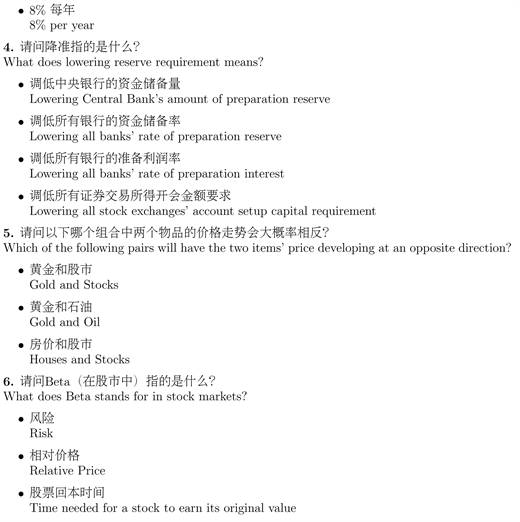
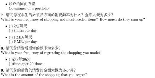
After collecting the results, I tried to quantify all the responses. Questions 1 and 10 focus the respondent’s family income overview and should be treated as basic demographic information. Questions 2 to 6 test the respondent’s level of financial literacy. Questions 7 to 9 are designed to assess the prudence of the respondent’s financial behaviors.

As we can categorize the questions into 3 types, I generate three separate indices named FLR, FBR and FWAL, representing for Financial Literacy Rate, Financial Behavior Rationality and Family Wealth Accumulation Level.

In the sensitivity analysis, we will directly put the raw data of all the question answers in the Financial Literacy assessment areas into the model as independent variables to eliminate the error that can be generated during the entropy weight defined procedure.

4. Statistical Models

Survey Responses Indices

As we may discern from the questionnaire attached in the appendix, the questions have defined correct answers and defined indicator of goodness¹.

We then define the variables FLR, FBR, and FWAL based on these questions. FLR is more like a test score. Based on the correctness of the answers to the Financial Literacy questions, we can define them as a quiz. In order to ensure to eliminate the luck part (those who choose by random and get the question right), I add in the following algorithm as shown in Equation (1):

$S_e=0=\frac{1}{I}\times W+\frac{I-1}{I}\times D$ (1)

S_e stands for the expected score of a single question if the respondent simply guesses it. I stands for the number of items for selection in the question.W stands for the score awarded for a correct answer. D stands for the score awarded for an incorrect answer.

Here we set the winning points to be 4. I is question specific, indicating that D is also specific to the question. For example, question 3 has three items to be chosen and only one correct answer. 4 points are won for a correct answer and 2 are deducted for an incorrect answer. Thus, the expected score is 0.

Therefore, we can discern that those who only guess all the questions will get an expected score of 0.

We should also consider the difficulty of each question. It is thus reasonable that we should use the Entropy Weight Model, as going to be explained in the next subsection.

Then we need to determine the value of FBR for each sample. FBR is defined as the rationality of the financial behavior of the respondent. Questions 7 to 9 account for the assessment of this variable. These questions has unlimited number of possible answers and are defined all as Minimal Indicators². Because we want to see an index in traditional sense, we process each response in for FBR as shown in Equation (2):

${x^{\prime }}_j=M_j-x_j$ (2)

And we will define $M_j$ in Equation (3):

$M_j=\underset{1\le i\le n}{\max }\left\{a_{ij}\right\}$ (3)

where $M_j$ is simply the largest value in the column.

After the process, we can discern that smaller the original value is, the larger the final value will be, satisfying to our requirement.

We can see that due to the fact that all the responses are of different dimensions and magnitudes, we need to eliminate these impacts. We then will conduct the normalization for the indicators of FBR, as shown in Equation (4).

$a_{ij}^{*}=\frac{a_{ij}}{\sqrt{{\displaystyle {\sum }_{i=1}^n{a}_{ij}^2}}}\left(i=1,2,\cdots ,n,1\le j\le m\right)$ (4)

After these processes, the variables can be changed from minimal indicators to larger indicators and then to indicators of equatable magnitude.

Next, we will again use Entropy Weight Model in order to settle down the weight of each factor to minimize the importance of the less varied determinants while magnify the importance of the more varied ones.

As for FWAL, we will define it as a row matrix with two columns. The first column will contain a value of 0 or 1. 0 indicates that the respondent’s family earn an income less than 50,000 RMB per year and should be classified in the less privileged group, as indicated by the Chinese Communist Party’s 5 Years’ Targets. 1 means that the income is more than 50,000 RMB annually and should be treated as wealthy. The second value is the percentage income increase of the family, being treated as the wealth accumulation increasing rate of the family. For a better illustration we will use the following Differential Equations, where W stands for the wealth occupied by the family:

$V_n=\frac{\text{d}W}{\text{d}t},Ar=\frac{\text{d}W}{\text{d}t}-2\%$ (5)

We define V_n as the nominal increasing rate of wealth. The accumulation rate Ar, on the other hand, should be defined as the increase in purchasing power over time, equaling V_n-CPI of the country. We will set the CPI for China as 2%.

In one word, for FWAL, the first column indicates which group, G_c or G_p, the respondent should be in with G_c refers to a common family while G_p refers to a wealthy family as defined by annual income.

Entropy Weight Model

Entropy characterizes the level of disorder and, to a large extent, the amount of information in a given system. In this case, the more randomness a variable displays, the higher its entropy and the faster its entropy increases, and so grows the amount of information we can extract from this variable.

The entropy weight method uses this principle to calculate weighting for different variables based on the entropy of their distributions. A larger variance or entropy generally means a larger weight. In the extreme case, if all values for a index are identical, then it does not matter what the value is, and we should give it zero weight.

TOPSIS Analysis

After getting all the needed indicator values for FLR and FBR, we can use the TOPSIS method to comprehensively evaluate each sample get their relative wellness.

We can get the best response group combination and the worst group combination, and evaluate using Kendall’s tau distance model (Jahanshahloo, Lotfi, & Izadikhah, 2006):

$\begin{array}{l}{D}_i^{+}=\sqrt{{\displaystyle {\sum }_{j=1}^m{w}_j{\left(Z_j^{+}-z_{ij}\right)}^2}}\\ D_i^{-}=\sqrt{{\displaystyle {\sum }_{j=1}^m{w}_j{\left(Z_j^{-}-z_{ij}\right)}^2}}\end{array}$ (6)

We can thus use the final evaluation equation:

$C_i=\frac{D_i^{-}}{D_i^{+}+D_i^{-}}$ (7)

The return value should be a value between 0 and 1.

Ordinary Least Square Regression Model

After obtaining the desired values for analysis, we sought out to determine correlation between one or more independent variables and one dependent variable. For convenience and other concerns defined FLR, we can simply use the two variable Ordinary Least Square Regression Model forFLR and FBR.

Now we will articulate our formulas for this model.

First, the general formula for OLS is shown in Equation (8):

$y_i={\beta }_1{x}_{i1}+{\beta }_2{x}_{i2}+\cdots +{\beta }_p{x}_{ip}+{\epsilon }_i$ (8)

where $y_i$ is the response variable; $\beta$ are the unknown variables; $x_i$ are the independent variables and ${\epsilon }_i$ is the unobserved error.

Significance Test Model

Next we should concentrate on the comparison between two income groups, G_c and G_p.

The two samples’ indices are FLR and FBR. To compare the two groups of pair values, we can simply use the Two Sample T-test.

To begin with, we will check whether each group satisfies the requirement for analysis using this method.

The samples can be treated as random for all respondents as the questionnaires are randomly selected. The sample is done without replacement. Luckily we should assume the sample size is far less than 10% of the whole population. Also the sample sizes are bigger than 30 for both samples. We thus satisfy the random and normal requirements.

As the true standard deviation of both income groups for FLR and FBR is unknown, we can use the sample standard error as a close approximation.

5. Model Results

We can compile all the calculated information for the entropy weight model into Figure 1 and Figure 2.

After getting the weights, we are able to use TOPSIS Method to evaluate. For brevity, the final results are available in the appendix. We display some examples of the values as classified by G_c and G_p in Figure 3.

Then we came to our OLS Regression Model. The model produced the following parameters, as shown in Table 1.

From the outcomes we can see that the regression model can only explain 14.72% of the observed values. However, the model is still functional because the F test shows that $F=87.524$ with $p=0.000<0.05$ , meaning that FLR definitely will affect FBR values.

The interpreted formula can be expressed as:

$F\hat{B}R=0.84-0.296FLR$ (9)

indicating a negative and significant relationship between the two variables, contradicting our assumption that as FLR increases, FBR will increase.

Figure 1. Entropy results for FLR.

Figure 2. Entropy results for FBR.

Figure 3. Entropy results for FBR.

Table 1. OLS regression results.

The p-value for the variable coefficient is 0.000, which is within a significance level as strict as 0.01, demonstrating that the negative correlation is almost certain.

Next, we will first compare the sample distribution in G_c and G_p.

We will use the two sample T-test for significance. The results are in Table 2.

Also we tested FBR in Table 3.

6. Sensitivity Analysis I

Wary of the low R² value for the OLS regression model, I decided to do a sensitivity analysis on it. This procedure includes testing the accountability of FBR on each respondent without the intermediate calculation of FLR.

The model shows the following results in Figure 4.

With these adjustments, R² is now higher and still shows an indication of correlation in terms of the F score.

7. Extension

7.1. Reflection

7.1.1. Results Deviation and Conformation

Deviation: The model results deviate from our expectations. We cannot confirm that:

Figure 4. OLS model output.

Table 2. T-test result for FLR in two groups.

Table 3. T-test result for FBR in two groups.

1) Young Adults living in privileged wealthy families will conduct more rationally in financial behaviors than the young from the common backgrounds.

2) Financial Literacy Rate will necessarily increase rationality of financial behaviors.

Conformation: However, one of the t-tests confirms the following hypothesis:

1) Young Adults living in privileged wealthy families have higher financial literacy rate than those in the common families.

We can aggregate the findings in one chart as in Figure 5.

The difference between the two groups’ two indices is clear.

Suspect: Some people may suggest that the wealth accumulation rate, Ar, will decrease the financial prudence of young adults. For responsibility, I will picture both variables in Figure 6.

Verification: For clarity, we will show the results of the tests only:

From this chart we can discern that Ar, the J in the chart, has no defined relationship with FBR.

7.1.2. Lurking Variables

Of common sense, increasing financial literacy will definitely increase one’s financial rationality. This leads us to wonder about the existence of lurking variables in this research.

We cannot conduct a controlled experiment in this area. Thus the most reasonable statistical account may be the following variables:

Figure 5. Group overall results.

Figure 6. Two variable distributions.

1) Households that can provide decent financial literacy education environment will have more stimuli to urge the young to conduct irrational purchases.

2) Parents in lower income households may offer less financial support for their children, thus prohibiting them from making financially irresponsible purchases.

It is a pity, but we cannot get conduct a controlled experiment due to time, financial and moral restrictions.

7.2. Psychological Explanation

Even though statistically we are almost done here, we can still account for the observed data using behavior finance and Gestalt Psychology.

7.2.1. Marginal Utility Theory

Excessive spending does not necessarily imply irrationality on the part of the consumer. Instead, we may consider that the consumer is rather buying “unnecessary” items in pursuit of a sense of fulfillment. In this sense, it is rightful that we should introduce the Marginal Utility Theory in Microeconomics. According to Marginal utility theory, “Utility is an idea that people get a certain level of satisfaction/happiness/utility from consuming goods and service” and “Marginal utility is the benefit of consuming an extra unit”.

Thus we can propose our theory:

• Marginal Utility Per Dollar for children of upper income households is less than for those of the middle and lower class backgrounds.

• To achieve the same amount of utility, young adults of wealthy households will purchase more.

• Necessary purchases for an individual have an identical dollar value regardless of his or her financial background.

• And thus the privileged young will purchase more “unnecessary” goods.

Still, unfortunately, it is only our postulation and cannot be verified using substantial statistics. However, the following suppositions can have some kind of supporting evidence.

7.2.2. Access to Confusing Purchasing Chances

Another factor we must consider is the effect of easy purchases and confusing advertisements.

We will set the following variables to quantify our assumption. Let T_i be the temptation coefficient of the product. P_i represents the probability of getting confused and buying the product, which depends on both FLR and T_i.

To simplify the model, we set three temptations of different degrees, being mild temptation, intermediate temptation and high temptation respectively. The consumer passes through these temptations daily, as demonstrated in Figure 7.

We set here that N1, N2, N3 should be 3, 2 and 1 respectively for young adults in wealthy families and will be 2, 1 and 0 for young adults in the less privileged families for their lack of access to such temptations in their living environment.

We are able to measure the effect of the differences in temptation coefficient for products and the number of temptations in the following simulations 7.3.

7.2.3. Theory of Planned Behaviors

By the concept of TPB, current behaviors are determined by past experiences and interactions. The young adults might base their purchasing behaviors on observed behavior of their parents. We could investigate the purchasing behavior of various parents and observe whether or not that correlates with the observed behavior of their children. Unfortunately, this research will have to be left to further surveys (Icek Ajzen, 2011).

Figure 7. Flow chart of temptations.

7.3. Statistical Simulation

Monte Carlo Simulation

Monte Carlo simulation is actually a general reference to an idea. As long as a large number of random samples are used when solving a problem, and then probabilistic analysis is performed on these samples, the method of predicting the results can be called a Monte Carlo method.

The idea for this model is that we will conduct numerous trials to simulate the process of living for the two groups and determine the average rate of purchasing unnecessary items.

Markov Chain Simulation

In the real world, there are many such phenomena: Under the condition that a certain system has known the current situation, the future state of the system is only related to the present, and the past history is not directly related. The mathematical model describing this kind of random phenomenon is called the Markov model.

In this situation, we will set an additional intermediate calculation in the program. This intermediate is affected by the former purchase of the day and will lower the probability of being lured by the same kind or higher level or temptation. An illustration is given below in Figure 8.

The equation form of the Markov Chain Model is:

$P\left\{{\xi }_{n+1}=j|{\xi }_n=i,{\xi }_{n-1}=i_{n-1},\cdots ,{\xi }_1=i_1\right\}=P\left\{{\xi }_{n+1}=j|{\xi }_n=i\right\}$ (10)

For clarity, the coding will be available in the appendix and the next section will present the model results directly.

7.4. Models Results

Table 4 is the summary of a simulations run for 1,000,000 iterations.³:

We can see our models do confirm that advertisements and easy access to payment is a factor in affecting FBR.

7.5. Additional Researches

To completely utilize my data, I conducted the following procedure. For brevity, I will present the statistical methods and results only briefly.

Population Estimation: Using a 99% confidence interval, we can state that we are we are 99% sure that the true population value for FLR and FBR will be contained by Table 5.

Differences with Confidence: 99% confidence intervals for the difference of the means of the indicators of both groups can be expressed, as shown in Table 6.

Table 4. Monte carlo results.

Figure 8. Flow chart of TPB.

Table 5. Population estimation.

Table 6. CI estimation.

7.6. Sensitivity Analysis II

We will vary the temptation rates in the simulation in order to test the sensitivity and significance of the tests.

Trail one: G_p 3:3:3 G_c 2:2:1,

Trial two: G_p 3:3:2 G_c 2:2:2.

The results show the same pattern as that in the previous tests, making FBR indicators lower for G_p than G_c.

8. Suggestions

No matter what the reason is, young adults from higher income households demonstrate more “irrational” shopping behavior. From the results of our statistical simulation, we can suspect that if we can change some of the variables in the test, the results can be improved. Sensitivity Analysis II was highly suggestive of our original hypotheses.

From these, we can propose the following suggestions to fight the observed lack of fiscal prudence of China’s young adults:

• Scrutinize advertisements,

• Offer more financial education to further increase the Financial Literacy Rate,

• Limit young adults’ access to online payment methods.

9. Conclusion

This article contains a plethora of statistical analyses. For brevity, lots of obscured and unnecessary procedures have been eliminated. However, to summarize the findings, we have included this chapter.

9.1. Outcomes

First of all, from the OLS and F test, we can see that the correlation between FLR and FBR is weak and possibly even unexpectedly negative.

Furthermore, young adults from less affluent households demonstrate an increased scrutiny of nonessential purchases when compared to their wealthier counterparts, as indicated in the significance test.

Finally, young adults from wealthier background have higher financial literacy rates than those from less privileged ones.

9.2. Suggestions

Some of our proposals for the cause of the unexpected results are not fit for implementation or need a further independent research to confirm. However, using statistical simulation methods, we have confirmed that advertisements and easy access to payment methods do increase a young adult’s theoretical likelihood of buying irresponsibly.

We thus propose that advertising should be further controlled to limit its sensational effects and that parents should limit their children’s access to mobile payments methods like Alipay in China.

Finally, we can see that financial literacy rate still plays a large role in determining the prudence of an individual’s spending behavior. For this reason, we as a society should continue to increase the availability of and access to financial education for all adults in China.

Special Thanks

This article is inspired by my Counselors, Erte Li at Wuxi Big Bridge Academy. He gave me phenomenal ideas and corresponding action guidelines. This paper could not have been realized without his help.

Thanks to those who responded to the questionnaires. It’s you who help to understand the financial behaviors now in China.

Acknowledgements

The survey that provided the data for analysis was conducted by an investigation group lead by the author, Muyan Xie, at Wuxi Big Bridge Academy International School Economics Club. As the president of the club, Muyan Xie leads his team to disseminate the survey. This paper was written solely by Muyan Xie.

Appendices

Questionnaire

Survey Data Chart

G_c Results

G_p Results

Coding (With corresponding images)

NOTES

¹This means that as the responses’ numerical values go down or up, it is clear whether the responses are good or bad, within a general trend.

²This means that as the responses going smaller and smaller, the better the response is.

³We automatically use the FLR acquired in the survey as parameters in the program; Temptation rates are set different for two groups, being 3:2:1 and 2:1:0 respectively. Other factors are set equal.

Conflicts of Interest

The authors declare no conflicts of interest regarding the publication of this paper.

References

[1]	Ajzen, I. (2011). The Theory of Planned Behaviour: Reactions and Reflections. Psychology & Health, 26, 1113-1127. https://doi.org/10.1080/08870446.2011.613995
[2]	Beutler, I. F., & Gudmunson, C. G. (2012). New Adolescent Money Attitude Scales: Entitlement and Conscientiousness. Journal of Financial Counseling and Planning, 23, 14. https://search.ebscohost.com/login.aspx?direct=true&db=psyh&AN=2013-08936-002&site=ehost-live&scope=site
[3]	Jahanshahloo, G. R., Lotfi, F. H., & Izadikhah, M. (2006). An Algorithmic Method to Extend TOPSIS for Decision-Making Problems with Interval Data. Applied Mathematics and Computation, 175, 1375-1384. https://doi.org/10.1016/j.amc.2005.08.048
[4]	Pillai, K. R., Carlo, R., & D’souza, R. (2012). Financial Prudence among Youth. Journal of Contemporary Management Research, 6, 52-68. https://search.ebscohost.com/login.aspx?direct=true&db=bth&AN=90299646&site=ehost-live&scope=site
[5]	Sharif, S. P. et al. (2020). Gender Differences in Financial Literacy and Financial Behaviour among Young Adults: The Role of Parents and Information Seeking. Journal of Family and Economic Issues, 41, 672-690. https://doi.org/10.1007/s10834-020-09674-z