On the Evaluation of Oscillatory Kind with Cauchy Principal Value

Changhao Li

Jinan University, Guangzhou, China.

DOI: 10.4236/jamp.2021.95067                

Abstract

In this paper, we discuss the integrals of oscillatory kind function with Cauchy principal value in point zero which have the form like , where f (x) is smooth function and r is odd integer. In this integral, x^r has several stationary points , and the Cauchy principal value . We use some integral technique to transform it into the form like  so that we can calculate it. At the end, we give some numerical examples to prove the accuracy of this method.

Keywords

Gauss-Quadrature, Cauchy Principal Value, Oscillatory Kind Function

1. Introduction

In this paper, we concerned about the Cauchy principal value in oscillatory kind function which $g\left(x\right)=x^r$, specifically have the form like

${\displaystyle {\int }_a^b\frac{f\left(x^r\right)e^{i\omega x^r}}{x}dx}$

where $f\left(x\right)$ is smooth and $\omega \in R$, generally $\omega$ is much large. Li [1] uses Levin method to solve the integral with Cauchy principal value. In that case, the principal value point is $\tau$ and $\tau \in [a,b]$, but the function $g\left(x\right)=x$. And the Levin method uses Chebyshev-Gauss-Labatt nodes to make a matrix equation in order to get the approximate solution. Then Wang [2] has mentioned a technique of put the integral to complex plane so that we can use a loop integral. In this paper, the author chooses several paths to make it available tot Gauss-Laguerre quadrature. It is a great idea for us to solve Cauchy principal value problem and we are using this idea to solve problem in this paper. Furthermore, Daan [3] puts forward the form of integral form. But in his paper, the integral without Cauchy principal value. Importantly, we take his idea of choose path, which make it easy to have a good path to integral. Alfrddo [4] then put the question to a more general situation. With the function $g\left(x\right)$ not smooth, maybe has stationary points and so on, they use Gauss-Fraud quadrature to solve the path near the stationary points.

In this paper, we firstly transformed the equation into the form which we known before, then we take the path to get the solution with Gauss-Laguerre quadrature. Finally two numerical examples are given to prove the method. One is for real part, and the other is for imaginary part.

2. Integral with Gauss-Laguerre Quadrature

As we can see, the variable x has a different order. First we need to transform x to let them have the same order. The specific process is

$\begin{array}{c}{\displaystyle {\int }_a^b\frac{f\left(x^r\right)e^{i\omega x^r}}{x}dx}={\displaystyle {\int }_a^b\frac{x^{r-1}f\left(x^r\right)e^{i\omega x^r}}{x{x}^{r-1}}dx}\\ =\frac{1}{r}{\displaystyle {\int }_a^b\frac{f\left(x^r\right)e^{i\omega x^r}}{x^r}d{x}^r}\\ =\frac{1}{r}{\displaystyle {\int }_{a^r}^{b^r}\frac{f\left(y\right)e^{i\omega y}}{y}dy}\end{array}$

In last equation, we use the variable substation of $y=x^r$ to transform it. The equation can be calculated in some methods like Li [1] has put forward.

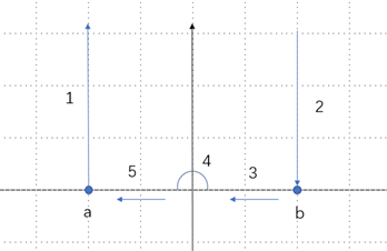
In such complex plane, the integral can be divided into several pieces which can be seen in above figure. Therefore, we only need to calculate the integral of path ${\Gamma }_1+{\Gamma }_2-{\Gamma }_4$ so that we can have the integral of path ${\Gamma }_3+{\Gamma }_5$.

The path ${\Gamma }_1$ and ${\Gamma }_3$ have similar situation. have mentioned a method about select a path to infinity as following

$g\left(h_x\left(p\right)\right)=g\left(x\right)+ip$

where $h_x\left(p\right)$ is the path start in x and end in infinity, $g\left(x\right)$ is the function $x^r$, and i is the imaginary unit, which is $\sqrt{-1}$, p is the variable. Now we prove the start point and the end point. Because $g\left(x\right)$ is smooth, so

$h_x\left(p\right)=g^{-1}\left(g\left(x\right)+ip\right)$

When $p=0$, $h_x\left(p\right)=x$, when $p\to \infty$, $h_x\left(p\right)\to \infty$. In this case, because of the known form of integral, the path can be written as following [3]

$h_x\left(p\right)=x+ip$

${h^{\prime }}_x\left(p\right)=i$

We need to notice that, p is the variable of $h_x\left(p\right)$, and x is the start point of the path.

Observe that

$\begin{array}{c}{\displaystyle {\int }_{{\Gamma }_1}\frac{f\left(y\right)e^{i\omega y}}{y}dy}={\displaystyle {\int }_0^{\infty }\frac{f\left(h_{-1}\left(p\right)\right)e^{i\omega h_{-1}\left(p\right)}}{h_{-1}(p)}d{h}_{-1}\left(p\right)}\\ ={\displaystyle {\int }_0^{\infty }\frac{f\left(-1+ip\right)e^{i\omega \left(-1+ip\right)}}{-1+ip}d\left(-1+ip\right)}\\ =\frac{i}{e^{i\omega }}{\displaystyle {\int }_0^{\infty }\frac{f\left(-1+ip\right)e^{-\omega p}}{-1+ip}dp}\\ =\frac{i}{e^{i\omega }}{\displaystyle {\int }_0^{\infty }\frac{f\left(-1+i\frac{q}{\omega }\right)e^{-q}}{-1+i\frac{q}{\omega }}d\frac{q}{\omega }}\\ =\frac{i}{\omega e^{i\omega }}{\displaystyle {\int }_0^{\infty }\frac{f\left(-1+i\frac{q}{\omega }\right)}{-1+i\frac{q}{\omega }}{e}^{-q}dq}\end{array}$

where $q=\omega p$ in the last equation.

The same

$\begin{array}{c}{\displaystyle {\int }_{{\Gamma }_2}\frac{f\left(y\right)e^{i\omega y}}{y}dy}={\displaystyle {\int }_0^{\infty }\frac{f\left(h_1\left(p\right)\right)e^{i\omega h_1\left(p\right)}}{h_1\left(p\right)}d{h}_1\left(p\right)}\\ =-\frac{i{e}^{i\omega }}{\omega }{\displaystyle {\int }_0^{\infty }\frac{f\left(1+i\frac{q}{\omega }\right)}{1+i\frac{q}{\omega }}{e}^{-q}dq}\end{array}$

We use polar coordinates to solve ${\Gamma }_4$. Let $y=r{e}^{i\theta }$, where r is the radio and θ is the variable.

$\begin{array}{c}{\displaystyle {\int }_{{\Gamma }_4}\frac{f\left(y\right)e^{i\omega y}}{y}dy}=-{\displaystyle {\int }_0^{\pi }\frac{f\left(r{e}^{i\theta }\right)e^{i\omega r{e}^{i\theta }}}{r{e}^{i\theta }}dr{e}^{i\theta }}\\ =-i{\displaystyle {\int }_0^{\pi }\frac{f\left(r{e}^{i\theta }\right)e^{i\omega r{e}^{i\theta }}}{r{e}^{i\theta }}r{e}^{i\theta }d\theta }\\ =-i{\displaystyle {\int }_0^{\pi }f\left(r{e}^{i\theta }\right)e^{i\omega r{e}^{i\theta }}d\theta }\end{array}$

When $r\to 0$, the equation above can be transformed into

${\displaystyle {\int }_{{\Gamma }_4}\frac{f\left(y\right)e^{i\omega y}}{y}dy}=-i\pi f(\; 0\; )$

As we discussed above, the integral () now can be written as following

$I\left[f\right]=i\pi f\left(0\right)+\frac{i{e}^{i\omega }}{\omega }{\displaystyle {\int }_0^{\infty }\frac{f\left(1+i\frac{q}{\omega }\right)}{1+i\frac{q}{\omega }}{e}^{-q}dq}+\frac{i}{\omega e^{i\omega }}{\displaystyle {\int }_0^{\infty }\frac{f\left(-1+i\frac{q}{\omega }\right)}{-1+i\frac{q}{\omega }}{e}^{-q}dq}$

Fortunately, the infinite integral can solve with Gauss-Laguerre quadrature with n-points. The $x_i$ represents Gauss-Laguerre points and the $w_i$ represents Gauss-Laguerre weights.

$I\left[f\right]\approx Q\left[f\right]=i\pi f\left(0\right)+\frac{i}{\omega e^{i\omega }}\underset{i=1}{\overset{\infty }{{\displaystyle \sum }}}{\omega }_i\frac{f\left(-1+i\frac{x_i}{{\omega }_i}\right)}{-1+i\frac{x_i}{{\omega }_i}}+\frac{i{e}^{i\omega }}{\omega }\underset{i=1}{\overset{\infty }{{\displaystyle \sum }}}{\omega }_i\frac{f\left(1+i\frac{x_i}{{\omega }_i}\right)}{1+i\frac{x_i}{{\omega }_i}}$

Remark 1 $Q\left[f\right]$ is the quadrature rule that we mentioned before with n points and weights. The approximation error behaves like

$I\left[f\right]-Q\left[f\right]=o\left({\omega }^{-2n-1}\right),\omega \to \infty$

3. Numerical Example

In order to prove this method is effective, we will use two examples to show the approximate solution and exact solution. All calculation is computed in Matlab2019a, and exact solution is given by Mathematica 12.0 with 64-digit.

Example1. The integral ${\displaystyle {\int }_{-1}^1{e}^{x^3}\frac{e^{i\omega x^3}}{x}dx}$ is analytic expression. Using above method, we can use $Q\left[f\right]$ to approach it which have the form like following

$Q\left[f\right]=i\pi +\frac{i}{\omega e^{i\omega }}\underset{i=1}{\overset{\infty }{{\displaystyle \sum }}}{\omega }_i\frac{f\left(-1+i\frac{x_i}{{\omega }_i}\right)}{-1+i\frac{x_i}{{\omega }_i}}+\frac{i{e}^{i\omega }}{\omega }\underset{i=1}{\overset{\infty }{{\displaystyle \sum }}}{\omega }_i\frac{f\left(1+i\frac{x_i}{{\omega }_i}\right)}{1+i\frac{x_i}{{\omega }_i}}$

Table 1 demonstrates the errors in real part. We can draw a conclusion that, with ω and n increasing, the accuracy of method is increasing. We take $\omega =16$ as example, when $n=5$ the results approach the max accuracy. When $\omega =32$, this process moves up when $n=4$.

Table 1. The real part error of ${\displaystyle {\int }_{-1}^1{e}^{x^3}\frac{e^{i\omega x^3}}{x}dx}$.

Table 2. The imaginary part error of ${\displaystyle {\int }_{-1}^1\cos (x^5)\frac{e^{i\omega x^5}}{x}dx}$.

Example 2. The integral of ${\displaystyle {\int }_{-1}^1\cos (x^5)\frac{e^{i\omega x^5}}{x}dx}$ only have imaginary part, so in this example, we can see the performance in imaginary part. This time we take $r=5$, and we still take $n=3,4,5$ to compare the efficiency about the method.

As we can see from Table 2, with n-points Gauss-Laguerre quadrature, the convergence is fast and only small n can obtain satisfying solution.

4. Conclusion

In this paper, we discuss the oscillatory kind function with Cauchy principal value which has a different form. The integral can be transformed into some known situation so that we can handle it easier. The method that puts the integral in complex plane in this paper comes from Wang [3] and the numerical solution is shown in Table 1 and Table 2. Within the two examples, we compare the real part and imaginary part between numerical solution and exact solution. And the absolute error represents the method for this integral is available.

Acknowledgements

The author would like to acknowledge to my tutor for teaching and useful discussion, and anonymous referees for suggestions.

Conflicts of Interest

The authors declare no conflicts of interest regarding the publication of this paper.

References

[1]	Li, J.B., Wang, X.S. and Wang, T. (2010) Evaluation of Cauchy Principal Value Integrals of Oscillatory Kind. Applied Mathematics and Computation, 217, 2390-2396. https://doi.org/10.1016/j.amc.2010.07.039
[2]	Wang, H.Y. and Xiang, S.H. (2009) On the Evaluation of Cauchy Principal Value Integrals of Oscillatory Functions. Journal of Computational and Applied Mathematics, 234, 95-100. https://doi.org/10.1016/j.cam.2009.12.007
[3]	Huybrechs, D. and Vandewalle, S. (2006) On the Evaluation of Highly Oscillatory Integrals by Analytic Continuation. SIAM Journal on Numerical Analysis, 44, 1026-1048. https://doi.org/10.1137/050636814
[4]	Deaño, A. and Huybrechs, D. (2009) Complex Gaussian Quadrature of Oscillatory Integrals. Numerische Mathematik, 112, 197-219. https://doi.org/10.1007/s00211-008-0209-z