The Assessment of After-Tax Performance

Andrew P. Leung

Independent Researcher, Melbourne, Australia.

DOI: 10.4236/jss.2021.94036                

Abstract

Over the years, the method of assessing an investment return after allowing for taxes has proved controversial, not least because the issue brings into sharp relief the different philosophies between active and passive fund management. This paper attempts to highlight the issues involved. After-tax performance may be defined generally as the return to an investor over a given time frame. Though many of the organizations and terminology are Australian, the concepts and tax systems are universal.

Keywords

After Tax Performance, Post-Liquidation, Pre-Liquidation, Active Management, Passive Management

1. Background

A common situation is for trustees or other fiduciaries to delegate the investment management of a portfolio of assets to professional or specialist managers. An example of such a situation is a superannuation fund, administered by a trustee. As the fund may have its own tax position, the trustee may enlist the help of managers by requiring them to target performance after tax in some fashion, in the hope of aligning the actions of the manager with the portfolio objectives of the trustee.

For example, this may occur where the asset allocation strategy of the portfolio is determined by the trustee, but the implementation of investment in particular asset classes is delegated to one or more specialist managers. In this event the tax position of the fund may be regarded as decentralized: each manager in its own way assists in meeting the trustee’s overall tax objectives.

How this can be achieved depends on the mandate agreed between the trustee and the particular manager. It may involve many issues, such as the realization of (deferred) tax credits, a bias towards imputation stocks, securities lending and so on. The design of mandates has to depend on the fund’s particular circumstances, and is beyond the scope of this paper.

However the most common situation that arises is where there are no tax complications, and the trustee simply wishes to assess how the after-tax performance of a manager compares with that of an agreed benchmark. This may be useful to the trustee in deciding, for example:

· the investment in a particular type of investment vehicle;

· the investment in a particular manager style; or

· the appointment of a particular manager.

The reason why after-tax performance is relevant is that an active manager may claim to add value on a before-tax basis, employing heavy trading of the investments under management. However there is an opportunity cost of heavy trading: early payment of Capital Gains Tax (CGT). The fund as a whole may be worse off if these costs are not allowed for. This paper addresses the fundamental and conceptual issues involved in after-tax performance assessment.

There are essentially two approaches to reporting after-tax performance: the pre-liquidation and post-liquidation approaches. Both have long histories and their own benefits and limitations. This paper supports the former approach from the viewpoint of assessment and monitoring of managers. The issue is given currency by regulation both approaches in both the US Bern Stein (1998), and in Australia Council (2018).

The issue is that the pre-liquidation philosophy and application is not well understood, and is thought to give a ‘free kick’ to passive managers and ETFs.

2. Framework

A common situation is for trustees or other fiduciaries to delegate the investment management of a portfolio of assets to professional or specialist managers. An example of such a situation is a superannuation fund, administered by a trustee. As the fund may have its own tax position, the trustee may enlist the help of managers by requiring them to target performance after tax in some fashion, in the hope of aligning the actions of the manager with the portfolio objectives of the trustee.

For example, this may occur where the asset allocation strategy of the portfolio is determined by the trustee, but the implementation of investment in particular asset classes is delegated to one or more specialist managers. In this event the tax position of the fund may be regarded as decentralized: each manager in its own way assists in meeting the trustee’s overall tax objectives.

How this can be achieved depends on the mandate agreed between the trustee and the particular manager. It may involve many issues, such as the realization of (deferred) tax credits, a bias towards imputation stocks, securities lending and so on. The design of mandates has to depend on the fund’s particular circumstances, and is beyond the scope of this paper.

However the most common situation that arises is where there are no tax complications, and the trustee simply wishes to assess how the after-tax performance of a manager compares with that of an agreed benchmark. This may be useful to the trustee in deciding, for example:

· the investment in a particular type of investment vehicle;

· the investment in a particular manager style; or

· the appointment of a particular manager.

The reason why after-tax performance is relevant is that an active manager may claim to add value on a before-tax basis, employing heavy trading of the investments under management. However there is an opportunity cost of heavy trading: early payment of Capital Gains Tax (CGT). The fund as a whole may be worse off if these costs are not allowed for. This paper addresses the fundamental and conceptual issues involved in after-tax performance assessment.

There are essentially two approaches to reporting after-tax performance: the pre-liquidation and post-liquidation approaches. Both have long histories and their own benefits and limitations. This paper supports the former approach from the viewpoint of assessment and monitoring of managers.

The issue is that the pre-liquidation philosophy and application is not well understood, and is thought to give a ‘free kick’ to passive managers and ETFs. For example, according to one active manager:

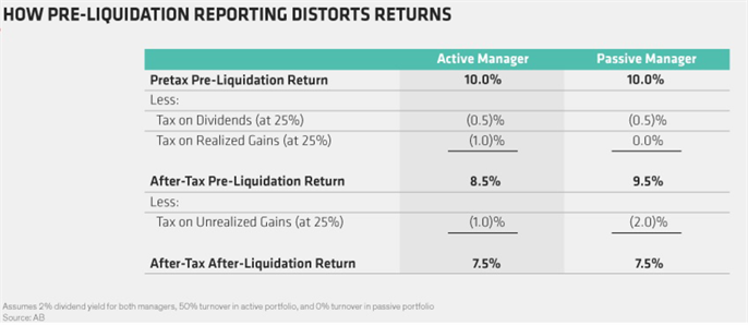
1) The pre-liquidation method assumes that the investor continues to hold fund shares at the end of the measurement period. In this method of reporting, after-tax returns are net of taxable distributions by the fund to its shareholders of dividends and capital gains realized through trading---but not of the capital gains taxes the investor will pay upon liquidation, as the Display below shows.

2) The post-liquidation method shows after-tax returns net of both distributions and the capital-gains taxes due upon liquidation. It more accurately reflects return after all taxes over the life of an investment.

3) Index funds trade very little, so their realized capital gains are very low. Actively managed funds trade more (sometimes, much more), so their realized gains are higher.

4) But most shareholders eventually sell their investments---and when they do, they have to pay taxes on the embedded capital gains. Because index funds don’t trade much, embedded gains tend to build to much higher levels over time. By contrast, the capital gains that actively managed funds distribute reduce the capital-gains taxes paid upon the eventual liquidation of the investment almost one for one.

To comment on the remarks above:

1) A statement of motherhood.

2) Another motherhood statement, which applies to both approaches. The term “accurately” is curious, since total taxes depend on the investment strategy involved.

3) See 3).

4) The implication is that active managers are not like most shareholders.

To understand the differences between the two approaches, it is necessary to consider their philosophy and underlying assumptions.

3. The Post-Liquidation Approach

A typical approach that has been advocated by active managers suggests that full provision for CGT on unrealized gains should be made in assessing performance. This approach is consistent with the accounting standards, which require tax expense to be based on CGT on both realized and unrealized gains during a year, to be reflected in net income as reported in the accounts.

A typical formula for assessing a manager’s after-tax return, such as that proposed by the P-Group is as follows:

$\begin{array}{l}\text{After}\text{tax}\text{return}\\ =\frac{1}{APV}\left[\left(RCG+UCG\right)\times \left[1-\left(1-d\right)t_s\right]+\left(OI+\frac{F{D}_A}{1-t_c}\right)\times \left(1-t_s\right)\right]\end{array}$ (1)

where during the period:

· RCG is realized capital gains;

· UCG is unrealized capital gains;

· $F{D}_A$ is franked dividends;

· OI is income other than franked dividends;

· APV is the average portfolio value;

· $t_c$ is the corporate tax rate applicable to franked dividends (i.e. 30%);

· $t_s$ is the investor’s tax rate (e.g. the superannuation rate of 15%);

· d is the CGT discount applicable to the investor (being $\frac{1}{3}$ for superannuation funds and life insurers, and $\frac{1}{2}$ for individuals).

The denominator APV should reflect the value of the asset portfolio at the start of the period, with full provision for tax on unrealized gains at that time. It should also give appropriate weighting to cash flows occurring during the period, including actual tax payments.

The above formula is based on the “discount” method of CGT, introduced in September 1999, applying to a fraction $1-d$ of nominal gains. For assets purchased before this date, the CGT may be based on the tax rate $t_s$ being applied fully to indexed gains.

The above formula effectively assumes that the entire portfolio is sold at the start of the measurement period, with CGT paid on the realized gains, and then the portfolio repurchased. A similar assumption is made at the end of the period. Thus this approach is said to be of post-liquidation type Mackenzie (2010).

A typical formula for assessing an after-tax benchmark return, consistent with the above return, is as follows:

$\begin{array}{l}\text{After}\text{tax}\text{benchmark}\text{return}\\ =\left\{\left[\frac{A{I}_1}{A{I}_0}-1\right]+\left[\frac{A{I}_1}{A{I}_0}-\frac{P{I}_1}{P{I}_0}\right]\times F{P}_L\times \frac{t_c}{1-t_c}\right\}\times \left(1-t_s\right)+\left[\frac{P{I}_1}{P{I}_0}-1\right]\times d\cdot t_s\end{array}$ (2)

where the symbols have the following meanings:

· $A{I}_0\mathrm{,}A{I}_1$ are the accumulation indexes at the start and end of the period respectively, so that $\frac{A{I}_1}{A{I}_0}-1$ is the total return over the period;

· $P{I}_0\mathrm{,}P{I}_1$ are the price indexes at the start and end of the period respectively, so that $\frac{P{I}_1}{P{I}_0}-1$ is the capital return over the period ;

· $\frac{A{I}_1}{A{I}_0}-\frac{P{I}_1}{P{I}_0}$ is thus the income return over the period, arising from dividends or other income;

· $F{P}_L$ is the average proportion of franked dividends¹ (zero in the case of overseas shares).

3.1. Comment on Post-Liquidation Approach

There are several shortcomings of the present framework in terms of both methodology and application.

1) The after tax benchmark is applicable, because it assumes that $1 of the liquidated portfolio at the start of the measurement period is fully invested in the index, which is then also liquidated at the end of the period. However this must apply equally for assessing the actual performance. The realized and unrealized gains, $RCG\mathrm{,}UCG$ and income $F{D}_A\mathrm{,}OI$ during the period in equation 1 are in practice generated by the assets before CGT is realized. However they should pertain to the liquidated assets APV, as depleted by payment of CGT. (In particular, tax on RCG should be assessed without any discount, if the measurement period is less than 12 months.) It is not clear that these adjustments are made in practice.

2) As the CGT on all gains, whether realized or unrealized, are brought into account in assessing after-tax returns, this mitigates the impact on managers who trade actively (as all assets are assumed to be liquidated at the end of the period).

3) Under the liquidation assumed by the P-Group it is not appropriate to compound on a time-weighted basis the after-tax returns for multiple periods. That would effectively assume sale and repurchase of assets several times This is a practical difficulty in presenting after-tax returns for periods of several years: under the post-liquidation approach the after-tax return assessed, and its benchmark, have to be specific to the period under consideration. Thus an after-tax benchmark series, say on a monthly basis, would not be feasible.

4) Taken to its logical extreme, the post-liquidation approach would remove the relevance of all legacy tax concessions. This is because the assumption of liquidation and repurchase puts CGT assessment on current terms, affecting such complications such as the following.

a) For securities purchased before September 1999, the better of the full tax rate on indexed gain or discounted rate on nominal gain applies;

b) t_s depends on what policy is adopted for realizing CGT, e.g. a FIFO approach, or an approach based on actual selection of scrip to be sold.

c) The CGT discount does not apply to gains made within 12 months of purchase.

This approach would therefore give little incentive to managers to manage these complications.

The conclusion that can be drawn from the above comments is that the present framework for assessing after-tax performance may possibly be adequate from the viewpoint of investor performance for specific periods, but is far from adequate in targeting certain aspects of managers’ performance and behaviour. These aspects are:

· The contribution to performance from active stock selection and trading;

· The choice of particular lines of stock to be sold, including with off-market buybacks;

· The realization of imputation credits and foreign tax credits.

4. The Pre-Liquidation Approach

It is apparent that the major issue with after-tax performance assessment is the treatment of CGT on unrealized gains, and to a much lesser extent the capture of imputation and foreign tax credits. The latter is essentially an issue of data, which should be dealt with by using precise levels of such credits in the assessment process.

The former issue is highly subjective as the value of CGT on unrealized gains depends on when they are realized. This is the same issue that affects unit pricing for unit trusts and PSTs, and there have been lengthy debates as to whether discounted or undiscounted provisions should be made for CGT. A consistent approach to this issue can, however, be developed by considering the choice of after-tax benchmark.

Benchmarks are invariably adopted as passive investment vehicles on a ‘buy and hold’ strategy. Passive managers aim to replicate such vehicles, and assert that one of the benefits of such an approach is the minimization of tax effects. If such an approach were ideally implemented, then gains would be realized only with changes in the index composition (as a result of the need to rebalance as new components are added or old ones removed). However, for investment of indefinite term in a passive vehicle, the liability to CGT on unrealized gains would be indefinitely deferred, and hence its impact would be minimal. This may be adopted as a simplifying (and probably close to realistic) assumption for performance assessment for long term investors.

In short, the pre-liquidation approach:

1) does not assume liquidation unless it actually occurs;

2) allows the CGT on non-liquidated assets to attract further investment return;

3) does not assume liquidation at the end of a reporting period, and therefore returns over contiguous periods may be “chained”.

On this basis, an after-tax benchmark return may be calculated as follows:

$\begin{array}{l}\text{After}\text{tax}\text{benchmark}\text{return}\\ =\left\{\left[\frac{A{I}_1}{A{I}_0}-1\right]+\left[\frac{A{I}_1}{A{I}_0}-\frac{P{I}_1}{P{I}_0}\right]\times F{P}_L\times \frac{t_c}{1-t_c}\right\}\times \left(1-t_s\right)+\left\{\frac{P{I}_1}{P{I}_0}-1\right\}\times t_s\end{array}$ (3)

which differs from that set out in Equation (2) only by adding back the full value (rather than the discounted value) of CGT on unrealized gains.

For consistency, it is necessary to disregard CGT on any unrealized gains in the calculation of actual after-tax performance:

$\text{After}\text{tax}\text{return}=\frac{1}{APV}\left[RCG+UCG+OI+F{D}_A-Tax\right]$ (4)

where Tax is the total actual tax payable during the period, after allowance for actual imputation credits and realized gains. Here APV does not need to be adjusted for CGT on unrealized gains that is, it may be based on the market value of assets at the start of the measurement period.

This approach is based on the value of unrealized CGT being zero, as the result of indefinite deferral, unless the manager decides to realize gains and incur CGT in practice (which is captured in Tax). Hence this approach is referred to as the pre-liquidation method.

The rationale behind the pre-liquidation method is not that gains will never be realized in practice. It is because the investor, and the manager, do not know when liquidation will be required, and they therefore have to assume that investment will be indefinite. The appropriate benchmark should therefore be a pre-liquidation index return.

Comments on Pre-Liquidation Approach

The pre-liquidation approach overcomes, or circumvents, all the practical shortcomings of the post-liquidation approach:

1) Since CGT on unrealized gains is effectively taken as zero, all the difficulties relating to the selection of the appropriate CGT basis are irrelevant (unless those decisions are actually made).

2) The actual CGT incurred on realized gains during the measurement period can be used directly in assessing performance. Such gains are generally at the control of the manager, and their impact is reflected in full.

3) It becomes possible to compound after-tax returns on the above basis over multiple periods, thereby simplifying the task of presenting performance results over multiple periods.

A possible disadvantage of the pre-liquidation approach is that the asset values to be used will differ from those shown in the investor’s accounts, because provision for CGT on unrealized gains will not be recognized. However it is rare for such inconsistency to be apparent in practice. In any event, the critical aspect is that after-tax performance and benchmarks should be measured consistently, which is fully achieved under the pre-liquidation approach.

The pre-liquidation approach has as long a history in assessing after-tax performance as the post-liquidation approach, although it may appear less intuitive. It has long underpinned the Global Investment Performance Standards (GIPS) of the CFA Institute AIMR (2011). In Australia, IFSA advocates disclosure on both a pre-liquidation as well as post-liquidation basis Financial Services Council (2008).

From the viewpoint of commercial providers, Morningstar provides a measure of tax effectiveness that uses the pre-liquidation approach exclusively Morningstar (2006). Index provider FTSE offers a series of global after-tax benchmarks FTSE (2010b) based on the pre-liquidation approach FTSE (2010c).

More recently, FTSE, in conjunction with ASFA, has introduced a series of Australian after-tax benchmarks. These are based on an approach where 1/5^th of the portfolio is turned over each year FTSE (2010a). They are thus in effect intermediate between the pre- and post-liquidation approaches. However they are not consistent with a truly passive investment style, under which turnover is triggered only by changes in the index composition.

The turnover on the S & P/ASX300 may be seen from the following table, for quarterly rebalancing on particular dates (Table 1).

The data is incomplete for 2005-2009. However, the data for the later years (by prorating the data for the periods less than a year for which it is available) provides the following liquidations to track the index (Table 2).

In other words, the liquidation required to track the S & P/ASX300 is much lower than 20%. Thus a true index manager could expect to outperform effortlessly the after-tax FTSE-ASFA indexes in the long term. This is not the hallmark of a meaningful after-tax benchmark.

5. After-Tax Valuation Approaches

It is sometimes suggested that the pre- and post-liquidation approaches to

Table 1. Total rebalancing on given dates.

Source: Vanguard, Goldman Sachs, S & P.

Table 2. ASX 300 liquidations.

after-tax performance are two extremes, neither of which ever holds in practice:

‘...some positive tax burden should be applied to unrealized gains because they are not untaxed but, rather, carry a contingent future tax liability’ ‘...measuring after-tax performance is an art form, rather than a science’ Rogers ‘Both methods may be unsatisfactory extremes. One method ignores accrued tax obligations, while the other immediately recognizes obligations that have not yet been paid and may not be paid for some time.’ (Horan et al., 2008)

The search for a compromise has been long and painful. Stein (1998) was the first to propose the concept of ‘After Tax Value’ (ATV) to serve as the basis for after-tax performance. Essentially ATV is the equivalent amount of cash which, when invested at the start of a given period, would give the same accumulation as an actual investment at the end of the period, after allowing for CGT. Naturally retrospective returns based on ATV are on a post-liquidation basis, calculated for the whole of the period (and all superannuation funds need to estimate deferred tax liabilities on such a basis). However ATVs are supposed to be assessed prospectively, before the end of the investment period.

Horan et al. (2008) provides an example of such a prospective valuation. It requires several assumptions, including:

· the intended period of the investment

· a consistent style of investment in relation to levels of dividends, income distributions, and realized gains

· the level of unrealized gains during the investment

· a risk adjusted discount rate for valuing the final accumulation.

Apart from possibly the first assumption, the others are subjective in nature. The last assumption is the most problematic, as it essentially requires a valuation methodology for the underlying investments. Horan et al. (2008) suggests a CAPM approach for the risk adjusted discount rate, which is effectively an attempt to second guess the market value for the assets.

Apart from possibly the first assumption, the others are subjective in nature. The last assumption is the most problematic, as it essentially requires a valuation methodology for the underlying investments. Horan et al. (2008) suggests a CAPM approach for the risk adjusted discount rate, which is effectively an attempt to second guess the market value for the assets.

Professional Standard 101 of the Actuaries Institute provides the following standard:

“.9 Treatment of Tax and Expenses STANDARD Presentation of investment performance must clearly state (a) before tax or after tax to indicate whether or not tax has been allowed for in the calculation. The calculation of after tax returns must adopt a consistent policy for the treatment of tax within each period. Where this treatment is changed, the effect of this change must be quantified.... ...Where comparisons of investment performance are presented, taxes (including tax benefits such as imputation credits) and fees must be treated on a consistent basis across all funds, benchmarks and managers included in the comparison unless it is impractical to make the necessary adjustments. In cases where it is not practical to make these adjustments, this must be noted and the differences between the bases used to calculate the figures should be explained.”

This standard does not in itself favor either the post- or pre-liquidation approach. However, as returns are usually compounded for reporting purposes, the pre-liquidation approach would be more logical to apply. The standard also appears to imply that assumptions involved as to future experience should be disclosed in investment comparisons. This is problematic for the ATV approach, which as discussed above requires a large number of such assumptions.

There is another approach, not dissimilar to the ATV in concept, but involving fewer assumptions. That is the use of deferred tax reserves (DTVs, or deferred tax benefits) in adjusting the valuation of assets. Though discounting of such reserves is not permitted by the accounting standards, APRA/ASIC sanction its use in unit pricing APRA (2008). The Actuaries Institute is non-committal on this issue, as it is related to unit pricing, not to performance assessment.

6. Fitness for Purpose

We now consider whether each of the performance assessment approaches discussed in this paper is appropriate and, if so, in what circumstances.

It should be clear from the preceding discussion that the feature that causes most difficulty in the assessment of after-tax performance is the period over which the performance is to be assessed.

This can be:

1) a specific period starting and ending in the past;

2) a specific period starting in the past or now, and ending at some specific future time;

3) an indefinite period starting in the past or now, and ending sometime in the future.

In the case of (1) there can be no argument that a post-liquidation basis is the most meaningful approach. Performance assessed in this case is for purely historical purposes, such as assessing the effects of asset allocation, or different investment vehicles. The issue (3) of Section 3.1 indicates that performance should be assessed for the whole of the period, and not compounded from sub-periods, as liquidation can take place only once, at the end of the period. Comparison of after-tax performance on this basis between different asset allocations, investment vehicles, manager styles, and managers is valid, if the responsibility for tax management has been delegated to the relevant investment fund. This includes comparison with benchmark or index funds which have similarly been treated for tax purposes.

In the case of (2), it is assumed that the manager or the investment fund is aware of the period of the investment (otherwise they cannot be held accountable for the tax implications arising from liquidation at the end of the period). Here the post-liquidation approach cannot be applied for the whole of the period (but may be applied for the period to date).

It is case (3) that is the most difficult, and probably the one that arises most often in practice.

7. The Case of Indefinite Commitment

Case (3) arises where neither the investor nor the manager knows the term of an investor’s commitment. It can also arise where the tax position of the assets can be transferred to another manager or vehicle without triggering CGT (i.e. CGT rollover relief is available). In this situation, it is the action of the investor to trigger CGT by liquidating the assets. The manager or fund should not be held accountable for this.

In this case, it is most meaningful to assume that the investment period is infinite. This has several advantages:

· it would allow the pre-liquidation approach to be justified, as liquidation is assumed never to occur;

· all the practical advantages of the pre-liquidation approach in Section 4 would apply, including the validity of compounding sub-period returns;

· it would allow direct comparison with index funds, for which CGT is minimal.

Published after-tax benchmarks, such as those introduced by FTSE, facilitate after-tax performance comparisons under this approach.

The practical issue which then arises is how to treat the liquidations that do actually occur, whether totally or partially, and whether at the request of the investor, or imposed involuntarily.

Adjustment for Involuntary Liquidation

To allow for liquidation of assets that is not at the control of the manager, the following adjustment may be made to remove CGT on involuntary liquidations:

$\begin{array}{l}\text{Adjusted}\text{after}\text{tax}\text{return}\\ =\frac{1}{APV}\left[RCG+UCG+OI+F{D}_A-Tax+CGT\times \frac{NW}{Sales}\right]\end{array}$

where:

· CGT is the total CGT payable in respect of liquidations during the period;

· Sales is the total proceeds from liquidation of assets during the period;

· NW is the net funds outflow during the period.

As a result of this adjustment, the after-tax performance of passive managers should be aligned with their benchmarks, unless there is significant change in the composition of their benchmarks, or they fail to replicate them.

8. Illustration of Various Approaches

In this section, we illustrate the application of the both the pre- and post-liquidation approaches for assessing after-tax performance set out in Section 7. This illustration is based on actual historical performance data for two managers, a passive manager in Australian equities, and an active manager in emerging markets equity for an 18 month period, together with their respective benchmarks.

The two managers’ markets are not directly comparable. No comparison between the managers is intended, nor indeed would it be relevant to the matters under consideration. The issue is how the managers perform in relation their respective benchmarks, and how that performance may be assessed. The illustration is provided solely to highlight the practical issues involved.

The issues that are considered in this illustration are whether:

1) the after-tax performance of the passive manager is closely aligned with its benchmark;

2) the trading costs of the active manager become more conspicuous under the pre-liquidation approach than under the post-liquidation approach;

3) the level of information required to implement after-tax performance assessment under the pre-liquidation approach can be feasibly provided on an ongoing basis.

8.1. After-Tax Performance under Post-Liquidation Approach

In Appendix A we set out details for the after-tax benchmarks and performance.

For the passive manager, the after-tax performance is reasonably in line with its after-tax benchmark.

For the active manager, it appears that after-tax performance has been slightly below benchmark for the period.

8.2. After-Tax Performance under Pre-Liquidation Approach

In Appendix B we set out the results of the after-tax performance assessment under the pre-liquidation approach.

For the passive manager, the results are not surprising. This confirms the manager’s status as a passive manager, with reasonably close tracking of its benchmark.

For the active manager, the results are in distinct contrast to those obtained under the post-liquidation approach. It significantly underperforms its benchmark.

8.3. Implications

In comparing the two managers’ after tax performance against their respective benchmarks, several interesting observations may be made.

Whilst compounding of monthly after-tax returns is not strictly justified under the post-liquidation basis, the final compounded statistic may be regarded simply as a summary of performance over the period given it is not intended a represent an after-tax return in its own right.

First the passive manager seems to track its benchmark closely over the period given, either on the pre- or post-liquidation basis. That is not surprising, because this manager seeks to replicate its benchmark, and any deviations would arise only from its method of replication and from cash flow effects.

Second, the choice of pre- or post-liquidation basis is much more critical for the active manager. Although it has performed reasonably close to its benchmark under the post-liquidation basis, its efforts in generating active returns have not evidently compensated for the opportunity cost of CGT, as realized early by such activities. This is precisely type of outcome that the pre-liquidation basis is designed to identify.

Another interesting feature is the relationship between the after-tax returns on the pre- and post-liquidation bases themselves. The actual returns for each manager are affected by the CGT actually incurred from month to month, as well as the active manager’s ability to add value. Hence a direct comparison of the returns on the two bases is not meaningful.

It is meaningful, however, to compare the benchmark returns under the two bases. A comparison of equation (2) and (3) indicates that the benchmarks differ only in the adjustment for the CGT discount factor d. If price movements are positive over a month, this would suggest the the pre-liquidation basis would produce a higher benchmark return than the post-liquidation basis, and vice versa if price movements are negative. This is consistent with the results set out in Appendices A and B.

9. Conclusion

This paper advocates the pre-liquidation approach to assessing after-tax performance where the investor’s commitment is indefinite, coupled with adjustment for involuntary liquidation. This closely reflects:

1) The way in which passive portfolios are managed to generate performance; and;

2) The way in which actual tax liabilities are incurred, rather than the way they are expensed for investors.

The pre-liquidation approach does not require any assumptions as to the investment style or to the level of turnover by the manager. The after-tax returns under this approach may be compounded over sub-periods in the same way as before-tax returns. However in practice this approach assumes that managers are not constrained by the cash flow position of the fund, and adjustments must be made if such constraints are imposed on the manager.

The illustration of this approach confirms that passive managers should not be significantly affected by the preferred approach since their transaction activity is expected to be low. However active managers may be significantly affected by the CGT liabilities they generate, which may tend to be camouflaged under tax accrual accounting. In the extreme case, a manager may turn over a portfolio every year, incurring actual tax liabilities, without deriving any active return from that trading. As the saying goes: ‘tax deferred is tax saved’. One of the benefits of after-tax performance assessment is to help identify managers who invest passively whilst charging active management fees.

The purpose of after-tax performance assessment is to quantify the success, or otherwise, provided by a fund manager in investing assets after allowing for the discretion provided to the manager in dealing with the tax consequences thereof. If the manager has full discretion in trading assets, then he must justify the advance payment constrained in particular areas, then his performance should be compared to a similar manager so constrained. The process then is of selecting an appropriate manager for comparison.

Appendix A. After-Tax Performance-Post-Liquidation Approach

Appendix B. After-Tax Performance-Pre-Liquidation Approach

NOTES

¹As available from data providers, such as Datastream.

Conflicts of Interest

The authors declare no conflicts of interest regarding the publication of this paper.

References

[1]	AIMR (2011). AIMR Performance Presentation Standards. Technical Report, CFA Institute. http://www.cfainstitute.org/ethics/Documents/Codes%20Documents/aftertax_changes.pdf
[2]	APRA (Australian Prudential Regulation Authority) (2008). Unit Pricing: Guide to Good Practice. Technical Report, APRA, ASIC. http://www.apra.gov.au
[3]	Council, F. S. (2018). Product Performance-Calculation of after-Tax Returns. Technical Report.
[4]	Financial Services Council (2008). Product performance-Calculation of after-Tax Returns. Technical Report, IFSA.
[5]	FTSE (2010a). FTSE ASFA Australia Index Series. Technical Report, FTSE.
[6]	FTSE (2010b). Ground Rules for the Management of the FTSE-ASFA Australia Index Series. Technical Report, FTSE.
[7]	FTSE (2010c). Guide to Calculation Methods for the FTSE Global Equity Index Series. Technical Report, FTSE.
[8]	Horan, S. M., Lawton, P. N., & Johnson, R. R. (2008). After-Tax Performance Measurement. The Journal of Wealth Management Summer, 11, 69-83. https://doi.org/10.3905/jwm.2008.706274
[9]	Mackenzie, G. D. (2010). Reporting Investment Performance after Tax. Technical Report, Atax, University of UNSW.
[10]	Morningstar (2006). After-Tax Performance Calculation Methodology. Technical Report, Morningstar.
[11]	Stein, D. M. (1998). Measuring and Evaluating Portfolio Performance after Taxes. The Journal of Portfolio Management Winter, 24, 117-124. https://www.sec.gov/rules/proposed/33-7809.htm https://doi.org/10.3905/jpm.24.2.117