Approximate Analytical Solutions to the Heat and Stokes Equations on the Half-Line Obtained by Fokas’ Transform

Mohamed Lachaab¹, Marius Beceanu²

¹University of Tunis, Tunis, Tunisia.
²University at Albany, New York, USA.

DOI: 10.4236/jamp.2021.94055                

Abstract

In this paper, we evaluate the integrals that are solutions of the heat and Stokes’ equations obtained by Fokas’ transform method by deriving exact formulas. Our method is more accurate and efficient than the contour deformation and parametrization used by Fokas to compute these integrals. In fact, for the heat equation, our solution is exact up to the imaginary error function and for the Stokes equation, our solution is exact up to the incomplete Airy function. In addition, our solutions extend to the lateral boundary without convergence issues, allow for asymptotic expansions, and are much faster than those obtained by other methods.

Keywords

Heat Equation, Stokes Equation, Fokas’ Transform, Asymptotic Expansion, Hilbert Transform, Incomplete Airy Function, Imaginary Error Function

1. Introduction

Fokas’ method (Fokas, 1997 [1] and 2002 [2] ) is a recently introduced approach that allows solving a large class of PDEs. Also known as the unified transform, this method extends classical approaches, such as separation of variables or the scattering transform, contains them as special cases, and gives solutions in situations where the classical methods cannot.

Classical methods work only poorly for spatial domains with boundary, when dealing with inhomogeneous boundary conditions. In this context, the key contribution of Fokas is the so-called “global relation”, which combines specified and unknown values of the solution and its derivatives on the boundary.

Fokas’ method gives the solutions as integrals on an unbounded contour in the complex plane. For example, for the heat and Stokes (first kind) equations on the half-line

$\begin{array}{l}{q}_t\left(x,t\right)-q_{xx}\left(x,t\right)=0,0<x<\infty ,0<t,\\ q\left(x,0\right)=q_0\left(x\right),0\le x,\\ q\left(0,t\right)=g_0\left(t\right),0\le t,\end{array}$ (1.1)

and

$\begin{array}{l}{q}_t\left(x,t\right)+q_{xxx}\left(x,t\right)=0,0<x<\infty ,0<t,\\ q\left(x,0\right)=q_0\left(x\right),0\le x,\\ q\left(0,t\right)=g_0\left(t\right),0\le t,\end{array}$ (1.2)

respectively, this method constructs the solutions $q\left(x\mathrm{,}t\right)$ as integrals (2.1) and (2.2) in the complex plane involving an x-transform of the initial condition $q_0$ and a t-transform of the boundary condition $g_0$ .

To evaluate these integrals numerically, Flyer-Fokas (2008, [3] ), Fokas et al. (2009, [4] ), and Papatheodorou-Kandili (2009, [5] ) used the steepest descent method, deforming the contour in the complex plane, then used the simple trapezoid rule, after parametrizing the curve, to compute the integral.

Following Flyer-Fokas [3] and for the sake of enabling a comparison, we make the choice

$q_0\left(x\right)=\mathrm{0,}{g}_0\left(t\right)=\sin \left(\lambda t\right)\mathrm{.}$

But, any reasonable (e.g. tempered distribution) Dirichlet boundary condition $g_0\left(t\right)$ can be decomposed into a superposition of sines, using the sine Fourier transform. Thus, we can solve the above equations for general boundary data. Initial data are simpler, to the point that one does not need Fokas’ method to handle them and will be treated elsewhere.

In this paper, we evaluate the integrals (2.1) and (2.2) by an alternative approach. First, we obtain a closed formula for the solution $q\left(x\mathrm{,}t\right)$ of the heat Equation (1.1) in terms of elementary functions and one special function, namely the imaginary error function erfi:

$q\left(x\mathrm{,}t\right)=\frac{{\text{e}}^{-\frac{x^2}{4t}}}{2}R\left[{\text{e}}^{-z_1^2}\left(i+\text{erfi}\left(-z_1\right)\right)+{\text{e}}^{-z_2^2}\left(i+\text{erfi}\left(-z_2\right)\right)\right]\mathrm{,}$

where $z_1$ and $z_2$ are defined later. Second, we obtain an exact expression for the solution of Stokes’ Equation (1.2) in terms of elementary functions and another special function, the incomplete Airy functions:

$q\left(x,t\right)=\frac{1}{2}\left(\sin \left(\lambda t+{\lambda }^{\frac{1}{3}}x\right)+{\text{e}}^{-\left(\frac{\sqrt{3}}{2}+\frac{i}{2}\right){\lambda }^{\frac{1}{3}}x}\sin \left(\lambda t\right)\right)+\frac{1}{4}{\displaystyle \underset{i=1}{\overset{6}{\sum }}}F\left({\alpha }_i^{*},x^{*}\right)$

where $F\left({\alpha }_i^{\mathrm{<mo>\; *\; </mo>}}\mathrm{,}{x}^{\mathrm{<mo>\; *\; </mo>}}\right)$ are functions of the incomplete Airy functions and will be determined later. The quantities $x^{\mathrm{<mo>\; *\; </mo>}}={\left(3t\right)}^{-\frac{1}{3}}x$ and ${\alpha }_i^{\mathrm{<mo>\; *\; </mo>}}={\left(3t\right)}^{\frac{1}{3}}{\alpha }_i$ .

The above formulas lend themselves well to applications, since there exist fast and highly accurate methods for computing the imaginary error function and incomplete Airy functions. For example, the imaginary error function is a standard function in MATLAB, where it is estimated with 10⁻²⁰ accuracy by means of Padé approximants (Cody, 1969 [6] ). Hence, our numerical solution is more accurate than Fokas’ solution and even than that of Papatheodorou-Kandili (2009, [5] ), who obtained a solution with 10⁻¹⁵ accuracy for the heat equation on a finite spatial domain. We also obtained speed improvements of at least an order of magnitude, see the Appendix A.

A related problem is that, as stated in Flyer-Fokas: “for $x=0$ , the integration interval is infinite and any truncation will result in the integral not converging exactly to the boundary condition”. By contrast, our exact expressions for the solutions extend all the way to the lateral boundary $x=0$ without this issue of convergence (they are still ill-behaved as $t\to 0$ , though).

In this paper, we also derive the asymptotic expansion for the heat equation solution with precise bounds for the error term, which allows one to compute the solution with arbitrarily high precision. This only requires evaluating elementary functions and the imaginary error function erfi.

The paper is organized as follows. In the next section, we briefly describe Fokas’ method as applied to Equations (1.1) and (1.2). In Section 3 we derive the exact formulas for the solutions. In Section 4 we obtain an asymptotic expansion for the heat equation solution, together with an estimate for the error size. Finally, in the Appendix B, we describe the numerical implementation of our scheme and compare the results to those of Flyer-Fokas.

2. Fokas’ Integral Solutions

In this section, we present the solutions of Equations (1.1) and (1.2) given by Fokas and that take the form of integrals. For the heat equation on the half-line with initial condition ( $q_0\left(x\right)=0$ ) and a Dirichlet boundary condition ( $g_0\left(t\right)=\sin \left(\lambda t\right)$ ), the solution is:

$q\left(x,t\right)=\frac{1}{2\pi }{\displaystyle {\int }_{\partial D^{+}}}\left(\frac{{\text{e}}^{-i\lambda t}-{\text{e}}^{-k^{2}t}}{k^2-i\lambda }-\frac{{\text{e}}^{i\lambda t}-{\text{e}}^{-k^{2}t}}{k^2+i\lambda }\right)k{\text{e}}^{ixk}\text{d}k$ (2.1)

For the Stokes’ equation of the first kind with the same initial and boundary conditions as above the solution is:

$q\left(x,t\right)=\frac{3}{4\pi }{\displaystyle {\int }_{\partial D^{+}}}\left(\frac{{\text{e}}^{i\lambda t}-{\text{e}}^{it{k}^3}}{\lambda -k^3}+\frac{{\text{e}}^{-i\lambda t}-{\text{e}}^{it{k}^3}}{\lambda +k^3}\right)k^2{\text{e}}^{ixk}\text{d}k$ (2.2)

To evaluate numerically these integrals, Flyer-Fokas (2008, [3] ) and Fokas et al., (2009, [4] ) deformed the contour of integration to a path in the region where the integrand decays exponentially fast for large k. Specifically, in order to get rapid convergence of the numerical scheme, they deformed the contour of integration to a hyperbola above the real axis and asymptotically below $\partial D^{+}$ . After that, they mapped the hyperbola from the complex plane to the real line using the following parametrisation:

$k\left(\theta \right)=i\gamma \sin \left(\alpha -i\theta \right)=\gamma \left(\cos \alpha \sinh \theta +i\sin \alpha \cosh \theta \right),$ (2.3)

which maps points $\theta$ on the real line to points $k\left(\theta \right)$ on a hyperbola in the complex plane. The integral in Equation (2.1) becomes (also see Formula (3.8) in Flyer-Fokas):

$q\left(x,t\right)=\frac{\gamma }{2\pi }{\displaystyle {\int }_{-\infty }^{\infty }}\left(\frac{{\text{e}}^{-i\lambda t}-{\text{e}}^{-k{\left(\theta \right)}^{2}t}}{k{\left(\theta \right)}^2-i\lambda }-\frac{{\text{e}}^{i\lambda t}-{\text{e}}^{-k{\left(\theta \right)}^{2}t}}{k{\left(\theta \right)}^2+i\lambda }\right)k\left(\theta \right){\text{e}}^{ixk\left(\theta \right)}\cos \left(\alpha -i\theta \right)\text{d}\theta .$ (2.4)

The parameters $\alpha$ and $\gamma$ were set to 1. After mapping the integral to the real line, Flyer-Fokas truncated the infinite integration interval to a finite one and used the simple trapezoidal rule. The same deformation-mapping procedure was used with the stokes Equation (2.2) except that $\alpha =\pi /8$ was replaced with $\pi /6$ .

$q\left(x,t\right)=\frac{3\gamma }{4\pi }{\displaystyle {\int }_{-\infty }^{\infty }}\left(\frac{{\text{e}}^{i\lambda t}-{\text{e}}^{ik{\left(\theta \right)}^{3}t}}{\lambda -k{\left(\theta \right)}^3}-\frac{{\text{e}}^{-i\lambda t}-{\text{e}}^{ik{\left(\theta \right)}^{3}t}}{\lambda +k{\left(\theta \right)}^3}\right)k{\left(\theta \right)}^2{\text{e}}^{ixk\left(\theta \right)}\cos \left(\alpha -i\theta \right)\text{d}\theta .$ (2.5)

3. Exact Formulas for the Solutions

3.1. The Heat Equation

Using several variables and contour changes, as well as Cauchy’s residue theorem, we obtain a more manageable expression for the solution $q\left(x,t\right)$ of the heat Equation (1.1). Our starting point is identity (2.1). Define the following four quantities $z_i$ , $1\le i\le 4$ , which will appear in the computation:

$z_{1,2,3,4}=i\frac{x}{2\sqrt{t}}+\sqrt[4]{-{\lambda }^2{t}^2}=\pm \sqrt{\frac{\lambda t}{2}}+i\left(\frac{x}{2\sqrt{t}}\pm \sqrt{\frac{\lambda t}{2}}\right).$

More precisely, let

$\begin{array}{l}{z}_1=-\sqrt{\frac{\lambda t}{2}}+i\left(\frac{x}{2\sqrt{t}}-\sqrt{\frac{\lambda t}{2}}\right),z_2=\sqrt{\frac{\lambda t}{2}}+i\left(\frac{x}{2\sqrt{t}}+\sqrt{\frac{\lambda t}{2}}\right),\\ z_3=-\sqrt{\frac{\lambda t}{2}}+i\left(\frac{x}{2\sqrt{t}}+\sqrt{\frac{\lambda t}{2}}\right),z_4=\sqrt{\frac{\lambda t}{2}}+i\left(\frac{x}{2\sqrt{t}}-\sqrt{\frac{\lambda t}{2}}\right).\end{array}$

They have the property that $z_1=-\overline{z_4}$ and $z_2=-\overline{z_3}$ . Consequently, $z_1^2=\overline{z_4^2}$ and $z_2^2=\overline{z_3^2}$ , We also note for future reference that

$z_1^2=-\frac{x^2}{4t}+x\sqrt{\frac{\lambda }{2}}-i\left(x\sqrt{\frac{\lambda }{2}}-\lambda t\right)=\overline{z_4^2},z_2^2=-\frac{x^2}{4t}-x\sqrt{\frac{\lambda }{2}}+i\left(x\sqrt{\frac{\lambda }{2}}+\lambda t\right)=\overline{z_3^2}.$

Lemma 3.1. The solution of Equation (1.1) is given by:

$q\left(x,t\right)=(\begin{array}{l}{\text{e}}^{-x\sqrt{\frac{\lambda }{2}}}\sin \left(\lambda t-x\sqrt{\frac{\lambda }{2}}\right)\\ -\frac{{\text{e}}^{-\frac{x^2}{4t}}}{4\pi }\left({\displaystyle {\sum }_{i=1}^2}{\displaystyle {\int }_{-\infty }^{+\infty }}\frac{{\text{e}}^{-k^2}}{k+z_i}\text{d}k-{\displaystyle {\sum }_{i=3}^4}{\displaystyle {\int }_{-\infty }^{+\infty }}\frac{{\text{e}}^{-k^2}}{k+z_i}\text{d}k\right),x<t\sqrt{2\lambda }\\ -\frac{{\text{e}}^{-\frac{\lambda t}{2}}}{4\pi }\left({\displaystyle {\sum }_{i=1}^2}{\displaystyle {\int }_{-\infty }^{+\infty }}\frac{{\text{e}}^{-k^2}}{k+z_i}\text{d}k-{\displaystyle {\sum }_{i=3}^4}{\displaystyle {\int }_{-\infty }^{+\infty }}\frac{{\text{e}}^{-k^2}}{k+z_i}\text{d}k\right),x=t\sqrt{2\lambda }\\ -\frac{{\text{e}}^{-\frac{x^2}{4t}}}{4\pi }\left({\displaystyle {\sum }_{i=1}^2}{\displaystyle {\int }_{-\infty }^{+\infty }}\frac{{\text{e}}^{-k^2}}{k+z_i}\text{d}k-{\displaystyle {\sum }_{i=3}^4}{\displaystyle {\int }_{-\infty }^{+\infty }}\frac{{\text{e}}^{-k^2}}{k+z_i}\text{d}k\right),x>t\sqrt{2\lambda }.\end{array}$ (3.1)

Proof. First, we convert the integral along the infinite contour to an integral on the real line. From (2.1), we have

$q\left(x,t\right)=\frac{1}{2\pi }{\displaystyle {\int }_{\partial D^{+}}}\left(\frac{{\text{e}}^{i\lambda t}\left(i\lambda k-k^3\right)+{\text{e}}^{-i\lambda t}\left(i\lambda k+k^3\right)-2i\lambda k{\text{e}}^{-t{k}^2}}{k^4+{\lambda }^2}\right){\text{e}}^{ixk}\text{d}k$ (3.2)

We consider the contour $C=\left[-R,R\right]\cup C_{R_2}\cup C_{\partial D^{+}}\cup C_{R_1}$ , where $C_{\partial D^{+}}$ is the part of C on the boundary of the domain $D^{+}$ and $C_{R_1}$ and $C_{R_2}$ are circular arcs of radius R. Let $f\left(k\right)$ denote the integrand. On the contour C there are two removable singularities at $k=\sqrt{i\lambda }$ and at $k=-\sqrt{-i\lambda }$ . There are no poles either inside or on the contour. Using the analyticity of the integrand, we have:

The contributions of the integrals along $C_{R_1}$ and $C_{R_2}$ vanish as $R\to \infty$ , by Jordan’s lemma. Equation (3.1) can be written as:

$q\left(x,t\right)=\frac{{\text{e}}^{-i\lambda t}}{2\pi }{\displaystyle {\int }_{\partial D^{+}}}\frac{k{\text{e}}^{ixk}}{k^2-i\lambda }\text{d}k-\frac{{\text{e}}^{i\lambda t}}{2\pi }{\displaystyle {\int }_{\partial D^{+}}}\frac{k{\text{e}}^{ixk}}{k^2+i\lambda }\text{d}k-\frac{i\lambda }{\pi }{\displaystyle {\int }_{\partial D^{+}}}\frac{k{\text{e}}^{-t{k}^2+ixk}}{k^4+{\lambda }^2}\text{d}k.$ (3.3)

Along $C_{R_1}$ , $k=R{\text{e}}^{i\theta }$ , for $0\le \theta \le \frac{\pi }{4}$ and $\text{d}k=Ri{\text{e}}^{i\theta }\text{d}\theta$ . The first integral in (3.3) becomes

${\displaystyle {\int }_0^{\frac{\pi }{4}}}\frac{R^{2}i{\text{e}}^{2i\theta }{\text{e}}^{ixR{e}^{i\theta }}}{R^2{\text{e}}^{2i\theta }-i\lambda }\text{d}\theta$

We will show that the integral of the modulus of the integrand converges to 0 as $R\to \infty$ and therefore the integral of the integrand converges to 0 as well.

$\left|{\displaystyle {\int }_0^{\frac{\pi }{4}}}\frac{R^{2}i{\text{e}}^{2i\theta }{\text{e}}^{ixR{e}^{i\theta }}}{R^2{\text{e}}^{2i\theta }-i\lambda }\text{d}\theta \right|\le {\displaystyle {\int }_0^{\frac{\pi }{4}}}\frac{R^2{\text{e}}^{-xR\sin \theta }}{\left|R^2{\text{e}}^{2i\theta }-i\lambda \right|}\text{d}\theta \le \frac{R^2}{R^2-\lambda }{\displaystyle {\int }_0^{\frac{\pi }{4}}}{\text{e}}^{-xR\sin \theta }\text{d}\theta$

Therefore, when $R\to \infty$ , the integral converges to 0 since $\sin \left(\theta \right)\ge 0$ for $0\le \theta \le \frac{\pi }{4}$ .

For the second integral in (3.3), we have

$\left|{\displaystyle {\int }_0^{\frac{\pi }{4}}}\frac{R^{2}i{\text{e}}^{2i\theta }{\text{e}}^{ixR{e}^{i\theta }}}{R^2{\text{e}}^{2i\theta }+i\lambda }\text{d}\theta \right|\le {\displaystyle {\int }_0^{\frac{\pi }{4}}}\frac{R^2{\text{e}}^{-xR\sin \theta }}{\left|R^2{\text{e}}^{2i\theta }+i\lambda \right|}\text{d}\theta \le {\displaystyle {\int }_0^{\frac{\pi }{4}}}\frac{R^2{\text{e}}^{-xR\sin \theta }}{\left|R^2{\text{e}}^{2i\theta }\right|}\text{d}\theta ={\displaystyle {\int }_0^{\frac{\pi }{4}}}{\text{e}}^{-xR\sin \theta }\text{d}\theta$

which also converges to 0 as $R\to \infty$ .

For the third integral, we have

$\begin{array}{c}\left|{\displaystyle {\int }_0^{\frac{\pi }{4}}}\frac{R{\text{e}}^{i\theta }{\text{e}}^{-t{R}^2{\text{e}}^{2i\theta }}{\text{e}}^{ixR{\text{e}}^{i\theta }}Ri{\text{e}}^{i\theta }}{R^4{\text{e}}^{4i\theta }+{\lambda }^2}\text{d}\theta \right|\le {\displaystyle {\int }_0^{\frac{\pi }{4}}}\frac{R^2{\text{e}}^{-t{R}^2\cos 2\theta -xR\sin \theta }}{\left|R^4{\text{e}}^{4i\theta }+{\lambda }^2\right|}\text{d}\theta \\ \le \frac{1}{R^2}{\displaystyle {\int }_0^{\frac{\pi }{4}}}{\text{e}}^{-t{R}^2\cos 2\theta -xR\sin \theta }\text{d}\theta \end{array}$

which converges to 0 as well as $R\to \infty$ since $\sin \left(\theta \right)\ge 0$ and $\cos \left(2\theta \right)\ge 0$ for $0\le \theta \le \frac{\pi }{4}$ .

Therefore, the three integrals vanish also along $C_{R_2}$ since $\sin \left(\theta \right)\ge 0$ and $\cos \left(2\theta \right)\ge 0$ for $\frac{3\pi }{4}\le \theta \le \pi$ . Also, as $R\to \infty$ , the contour $C_{\partial D^{+}}$ becomes $-\partial D^{+}$ . Therefore, as $R\to \infty$ ,

${\displaystyle {\int }_{\partial D^{+}}}f\left(k\right)\text{d}k={\displaystyle {\int }_{-\infty }^{\infty }}f\left(k\right)\text{d}k.$

and,

$q\left(x,t\right)=\frac{{\text{e}}^{-i\lambda t}}{2\pi }{\displaystyle {\int }_{-\infty }^{+\infty }}\frac{k{\text{e}}^{ixk}}{k^2-i\lambda }\text{d}k-\frac{{\text{e}}^{i\lambda t}}{2\pi }{\displaystyle {\int }_{-\infty }^{+\infty }}\frac{k{\text{e}}^{ixk}}{k^2+i\lambda }\text{d}k-\frac{i\lambda }{\pi }{\displaystyle {\int }_{-\infty }^{+\infty }}\frac{k{\text{e}}^{-t{k}^2+ixk}}{k^4+{\lambda }^2}\text{d}k.$ (3.4)

Now, we evaluate each of these three integrals. The first and second one are computed directly using the residue theorem. The third one is computed using a different strategy.

For the first integral, we consider a contour that is the boundary of an upper semicircular region of a circle of a radius large enough to include the pole $\sqrt{i\lambda }$ . Using the residue theorem and Jordan’s lemma, we get:

$\frac{{\text{e}}^{-i\lambda t}}{2\pi }{\displaystyle {\int }_{-\infty }^{+\infty }}\frac{k{\text{e}}^{ixk}}{k^2-i\lambda }\text{d}k=\left(\frac{{\text{e}}^{-i\lambda t}}{2\pi }\right)2\pi i\text{Res}\left(\sqrt{i\lambda }\right)=\frac{i}{2}{\text{e}}^{-x\sqrt{\frac{\lambda }{2}}+i\left(x\sqrt{\frac{\lambda }{2}}-\lambda t\right)}$ (3.5)

In this integral, we need not consider the residue at the other pole $-\sqrt{i\lambda }$ since it is not inside the contour. Same holds for the second integral. We consider a contour that is the boundary of an upper semicircular region of a circle of radius large enough to include the pole $-\sqrt{-i\lambda }$ . Using the residue theorem, we get:

$\begin{array}{l}\frac{{\text{e}}^{i\lambda t}}{2\pi }{\displaystyle {\int }_{-\infty }^{+\infty }}\frac{k{\text{e}}^{ixk}}{k^2+i\lambda }\text{d}k=\frac{i}{2}{\text{e}}^{-x\sqrt{\frac{\lambda }{2}}-i\left(x\sqrt{\frac{\lambda }{2}}-\lambda t\right)}\hfill \end{array}$ (3.6)

In this integral as well, we need not consider the residue at the other pole $\sqrt{-i\lambda }$ since it is not inside the contour. Summing (3.5) and (3.6) gives:

$\frac{{\text{e}}^{-i\lambda t}}{2\pi }{\displaystyle {\int }_{-\infty }^{+\infty }}\frac{k{\text{e}}^{ixk}}{k^2-i\lambda }\text{d}k-\frac{{\text{e}}^{i\lambda t}}{2\pi }{\displaystyle {\int }_{-\infty }^{+\infty }}\frac{k{\text{e}}^{ixk}}{k^2+i\lambda }\text{d}k=-{\text{e}}^{-x\sqrt{\frac{\lambda }{2}}}\sin \left(x\sqrt{\frac{\lambda }{2}}-\lambda t\right)$ (3.7)

For the third integral in (3.4), we use the partial fractions decomposition of $\frac{k}{k^4+{\lambda }^2}$ as:

$\frac{k}{k^4+{\lambda }^2}=\frac{1}{4\lambda i}\left(\frac{1}{k-\sqrt{i\lambda }}+\frac{1}{k+\sqrt{i\lambda }}-\frac{1}{k-\sqrt{-i\lambda }}-\frac{1}{k+\sqrt{-i\lambda }}\right)\mathrm{.}$ (3.8)

We get:

$\begin{array}{c}-\frac{i\lambda }{\pi }{\displaystyle {\int }_{-\infty }^{+\infty }}\frac{k{\text{e}}^{-t{k}^2+ixk}}{k^4+{\lambda }^2}\text{d}k=\frac{-1}{4\pi }({\displaystyle {\int }_{-\infty }^{+\infty }}\frac{{\text{e}}^{-t{k}^2+ixk}}{k-\sqrt{i\lambda }}\text{d}k+{\displaystyle {\int }_{-\infty }^{+\infty }}\frac{{\text{e}}^{-t{k}^2+ixk}}{k+\sqrt{i\lambda }}\text{d}k\\ -{\displaystyle {\int }_{-\infty }^{+\infty }}\frac{{\text{e}}^{-t{k}^2+ixk}}{k-\sqrt{-i\lambda }}\text{d}k-{\displaystyle {\int }_{-\infty }^{+\infty }}\frac{{\text{e}}^{-t{k}^2+ixk}}{k+\sqrt{-i\lambda }}\text{d}k)\end{array}$ (3.9)

We next compute these four integrals. After changing the variable k by $\tilde{k}=k\sqrt{t}$ and completing the square in $\tilde{k}$ , we have:

• The first integral

${\displaystyle {\int }_{-\infty }^{+\infty }}\frac{{\text{e}}^{-t{k}^2+ixk}}{k-\sqrt{i\lambda }}\text{d}k={\text{e}}^{-\frac{x^2}{4t}}{\displaystyle {\int }_{-\infty }^{+\infty }}\frac{{\text{e}}^{-{\left(\tilde{k}-i\frac{x}{2\sqrt{t}}\right)}^2}}{\tilde{k}-\sqrt{i\lambda }\sqrt{t}}\text{d}\tilde{k},$

Another change of variable: $k=\tilde{k}-i\frac{x}{2\sqrt{t}}$ , gives:

${\displaystyle {\int }_{-\infty }^{+\infty }}\frac{{\text{e}}^{-t{k}^2+ixk}}{k-\sqrt{i\lambda }}\text{d}k={\text{e}}^{-\frac{x^2}{4t}}{\displaystyle \underset{-\infty -i\frac{x}{2\sqrt{t}}}{\overset{+\infty -i\frac{x}{2\sqrt{t}}}{\int }}}\frac{{\text{e}}^{-k^2}}{k+z_1}\text{d}k,$ (3.10)

where $z_1=i\frac{x}{2\sqrt{t}}-\sqrt{i\lambda }\sqrt{t}=-\sqrt{\frac{\lambda t}{2}}+i\left(\frac{x}{2\sqrt{t}}-\sqrt{\frac{\lambda t}{2}}\right)$ .

The integrand in the right hand side of (3.10) has $-z_1$ as a pole. Deforming the integral back to the real line will result in a residue at $-z_1$ exactly when

$\mathrm{Im}\left(-z_1\right)=\sqrt{\frac{\lambda t}{2}}-\frac{x}{2\sqrt{t}}$ is non-positive (Cauchy’s theorem). If $x\ge t\sqrt{2\lambda }$ , then there is a residue. If $x<t\sqrt{2\lambda }$ , then the pole is not inside the contour. Therefore, the first integral is:

${\displaystyle {\int }_{-\infty }^{+\infty }}\frac{{\text{e}}^{-t{k}^2+ixk}}{k-\sqrt{i\lambda }}\text{d}k=\{\begin{array}{l}{\text{e}}^{-\frac{x^2}{4t}}{\displaystyle {\int }_{-\infty }^{+\infty }}\frac{{\text{e}}^{-k^2}}{k+z_1}\text{d}k,x<t\sqrt{2\lambda }\\ {\text{e}}^{-\frac{x^2}{4t}}{\displaystyle {\int }_{-\infty }^{+\infty }}\frac{{\text{e}}^{-k^2}}{k+z_1}\text{d}k+\pi i\text{Res}\left(-z_1\right),x=t\sqrt{2\lambda }\\ {\text{e}}^{-\frac{x^2}{4t}}{\displaystyle {\int }_{-\infty }^{+\infty }}\frac{{\text{e}}^{-k^2}}{k+z_1}\text{d}k+2\pi i\text{Res}\left(-z_1\right),x>t\sqrt{2\lambda },\end{array}$

where the integral is interpreted in the principal value sense when $z_1\in ℝ$ and

$\text{Res}\left(-z_1\right)=\underset{k\to -z_1}{lim}{\text{e}}^{-\frac{x^2}{4t}}\left(k+z_1\right)\frac{{\text{e}}^{-k^2}}{k+z_1}={\text{e}}^{-\frac{x^2}{4t}-z_1^2}={\text{e}}^{-x\sqrt{\frac{\lambda }{2}}+i\left(x\sqrt{\frac{\lambda }{2}}-\lambda t\right)}.$ (3.11)

• The second integral

${\displaystyle {\int }_{-\infty }^{+\infty }}\frac{{\text{e}}^{-t{k}^2+ixk}}{k+\sqrt{i\lambda }}\text{d}k={\text{e}}^{-\frac{x^2}{4t}}{\displaystyle {\int }_{-\infty }^{+\infty }}\frac{{\text{e}}^{-k^2}}{k+z_2}\text{d}k,$

where $z_2=\sqrt{\frac{\lambda t}{2}}+i\left(\frac{x}{2\sqrt{t}}+\sqrt{\frac{\lambda t}{2}}\right)$ . Note that in this case there is no residue

associated with the pole $-z_2$ since it is outside the contour when deforming the integral to the real line.

• The third integral

${\displaystyle {\int }_{-\infty }^{+\infty }}\frac{{\text{e}}^{-t{k}^2+ixk}}{k-\sqrt{-i\lambda }}\text{d}k={\text{e}}^{-\frac{x^2}{4t}}{\displaystyle {\int }_{-\infty }^{+\infty }}\frac{{\text{e}}^{-k^2}}{k+z_3}\text{d}k,$

where $z_3=-\sqrt{\frac{\lambda t}{2}}+i\left(\frac{x}{2\sqrt{t}}+\sqrt{\frac{\lambda t}{2}}\right)$ . Note also that deforming the integral on the

real line in this case will not result in a residue since the pole $-z_3$ is never inside the contour.

• The fourth integral

${\displaystyle {\int }_{-\infty }^{+\infty }}\frac{{\text{e}}^{-t{k}^2+ixk}}{k+\sqrt{-i\lambda }}\text{d}k=\{\begin{array}{l}{\text{e}}^{-\frac{x^2}{4t}}{\displaystyle {\int }_{-\infty }^{+\infty }}\frac{{\text{e}}^{-k^2}}{k+z_4}\text{d}k,x<t\sqrt{2\lambda }\\ {\text{e}}^{-\frac{x^2}{4t}}{\displaystyle {\int }_{-\infty }^{+\infty }}\frac{{\text{e}}^{-k^2}}{k+z_4}\text{d}k+\pi i\text{Res}\left(-z_4\right),x=t\sqrt{2\lambda }\\ {\text{e}}^{-\frac{x^2}{4t}}{\displaystyle {\int }_{-\infty }^{+\infty }}\frac{{\text{e}}^{-k^2}}{k+z_4}\text{d}k+2\pi i\text{Res}\left(-z_4\right),x>t\sqrt{2\lambda },\end{array}$

where $z_4=\sqrt{\frac{\lambda t}{2}}+i\left(\frac{x}{2\sqrt{t}}-\sqrt{\frac{\lambda t}{2}}\right)$ . Deforming the integral on the real line will

result in a residue depending on the location of the pole $-z_4$ . The residue at $-z_4$ is:

$\text{Res}\left(-z_4\right)=\underset{k\to -z_4}{lim}{\text{e}}^{-\frac{x^2}{4t}}\left(k+z_4\right)\frac{{\text{e}}^{-k^2}}{k+z_4}={\text{e}}^{-\frac{x^2}{4t}-z_4^2}={\text{e}}^{-x\sqrt{\frac{\lambda }{2}}-i\left(x\sqrt{\frac{\lambda }{2}}-\lambda t\right)}.$ (3.12)

The difference of the residues at $-z_1$ and $-z_4$ is

$\text{Res}\left(-z_1\right)-\text{Res}\left(-z_4\right)={\text{e}}^{-\frac{x^2}{4t}}\left({\text{e}}^{-z_1^2}-{\text{e}}^{-z_4^2}\right)=2i{\text{e}}^{-x\sqrt{\frac{\lambda }{2}}}\sin \left(x\sqrt{\frac{\lambda }{2}}-\lambda t\right),$

which cancels in the boundary case $x=t\sqrt{2\lambda }$ . Therefore, the sum of (3.7) and (3.9) produces (3.1), which is what we wanted to prove. $\square$

We note that

$F\left(z\right)={\displaystyle {\int }_{-\infty }^{+\infty }}\frac{{\text{e}}^{-k^2}}{k+z}\text{d}k.$

is odd and $F\left(\bar{z}\right)=\overline{F\left(z\right)}$ . Since $z_1=-\overline{z_4}$ and $z_2=-\overline{z_3}$ , it follows that $F\left(z_4\right)=-\overline{F\left(z_1\right)}$ and $F\left(z_3\right)=-\overline{F\left(z_2\right)}$ . Then

${\displaystyle \underset{i=1}{\overset{2}{\sum }}}{\displaystyle {\int }_{-\infty }^{+\infty }}\frac{{\text{e}}^{-k^2}}{k+z_i}\text{d}k-{\displaystyle \underset{i=3}{\overset{4}{\sum }}}{\displaystyle {\int }_{-\infty }^{+\infty }}\frac{{\text{e}}^{-k^2}}{k+z_i}\text{d}k=2R{\displaystyle \underset{i=1}{\overset{2}{\sum }}}{\displaystyle {\int }_{-\infty }^{+\infty }}\frac{{\text{e}}^{-k^2}}{k+z_i}\text{d}k.$ (3.13)

Therefore Equation (3.1) becomes:

$q\left(x,t\right)=(\begin{array}{l}{\text{e}}^{-x\sqrt{\frac{\lambda }{2}}}\sin \left(\lambda t-x\sqrt{\frac{\lambda }{2}}\right)-\frac{{\text{e}}^{-\frac{x^2}{4t}}}{2\pi }R{\displaystyle {\sum }_{i=1}^2}{\displaystyle {\int }_{-\infty }^{+\infty }}\frac{{\text{e}}^{-k^2}}{k+z_i}\text{d}k,x<t\sqrt{2\lambda }\\ -\frac{{\text{e}}^{-\frac{\lambda t}{2}}}{2\pi }R{\displaystyle {\sum }_{i=1}^2}{\displaystyle {\int }_{-\infty }^{+\infty }}\frac{{\text{e}}^{-k^2}}{k+z_i}\text{d}k,x=t\sqrt{2\lambda }\\ -\frac{{\text{e}}^{-\frac{x^2}{4t}}}{2\pi }R{\displaystyle {\sum }_{i=1}^2}{\displaystyle {\int }_{-\infty }^{+\infty }}\frac{{\text{e}}^{-k^2}}{k+z_i}\text{d}k,x>t\sqrt{2\lambda }.\end{array}$ (3.14)

3.2. The Stokes Equation of the First Kind

Lemma 3.2. The solution of Equation (1.2) is given by:

$q\left(x,t\right)=\frac{1}{2}\left(\sin \left(\lambda t+{\lambda }^{\frac{1}{3}}x\right)+{\text{e}}^{-\left(\frac{\sqrt{3}}{2}+\frac{i}{2}\right){\lambda }^{\frac{1}{3}}x}\sin \left(\lambda t\right)\right)+\frac{1}{4\pi }{\displaystyle \underset{i=1}{\overset{6}{\sum }}}{\displaystyle {\int }_{ℝ}}\frac{{\text{e}}^{i\left(t{k}^3+xk\right)}}{k-{\alpha }_i}\text{d}k.$ (3.15)

where ${\alpha }_1={\lambda }^{\frac{1}{3}}$ , ${\alpha }_2=-{\lambda }^{\frac{1}{3}}\in ℝ$ ; ${\alpha }_3=\left(\frac{1}{2}+i\frac{\sqrt{3}}{2}\right){\lambda }^{\frac{1}{3}}$ , ${\alpha }_4=\left(-\frac{1}{2}+i\frac{\sqrt{3}}{2}\right){\lambda }^{\frac{1}{3}}\in {ℂ}^{+}$ ; ${\alpha }_5=\left(\frac{1}{2}-i\frac{\sqrt{3}}{2}\right){\lambda }^{\frac{1}{3}}$ , ${\alpha }_6=\left(-\frac{1}{2}-i\frac{\sqrt{3}}{2}\right){\lambda }^{\frac{1}{3}}\in {ℂ}^{-}$ .

Proof. From Equation (2.2), we have that

$q\left(x,t\right)=\frac{3}{4\pi }{\displaystyle {\int }_{\partial D^{+}}}{\text{e}}^{ixk}\left(\frac{{\text{e}}^{i\lambda t}\left(\lambda k^2+k^5\right)+{\text{e}}^{-i\lambda t}\left(\lambda k^2-k^5\right)-2k^5{\text{e}}^{it{k}^3}}{{\lambda }^2-k^6}\right)\text{d}k.$ (3.16)

We convert the integral along the infinite contour to an integral on the real line. Consider the contour $C=\left[-R,R\right]\cup C_{R_1}\cup C_{\partial D^{+}}\cup C_{R_2}$ , where $C_{\partial D^{+}}$ is the part of C on the boundary of the domain $D^{+}$ and $C_{R_1}$ and $C_{R_2}$ are circular arcs of radius R. Let $f\left(k\right)$ denote the integrand. On the contour C, there are

four poles: $k_1={\lambda }^{\frac{1}{3}}$ , $k_2=-{\lambda }^{\frac{1}{3}}$ , $k_3=\left(\frac{1}{2}+i\frac{\sqrt{3}}{2}\right){\lambda }^{\frac{1}{3}}$ and $k_4=\left(-\frac{1}{2}+i\frac{\sqrt{3}}{2}\right){\lambda }^{\frac{1}{3}}$ . Using the analyticity of the integrand, we obtain:

$\begin{array}{c}{\displaystyle {\oint }_C}f\left(k\right)\text{d}k={\displaystyle {\int }_{-R}^R}f\left(k\right)\text{d}k+{\displaystyle {\int }_{C_{R_1}}}f\left(k\right)\text{d}k+{\displaystyle {\int }_{C_{\partial D^{+}}}}f\left(k\right)\text{d}k+{\displaystyle {\int }_{C_{R_2}}}f\left(k\right)\text{d}k\\ =\pi i\left\{\text{Res}\left(k_1\right)+\text{Res}\left(k_2\right)+2\text{Res}\left(k_3\right)+2\text{Res}\left(k_4\right)\right\}\\ =0,\end{array}$

because the residues at $k_1$ , $k_2$ , $k_3$ and $k_4$ are all equal to 0. (It is easy to show that. The proof is available upon request).

The contributions of the integral vanish along $C_{R_1}$ and $C_{R_2}$ . In fact, $q\left(x\mathrm{,}t\right)$ can be written as:

$q\left(x,t\right)=\frac{3}{4\pi }{\text{e}}^{i\lambda t}{\displaystyle {\int }_{ℝ}}\frac{k^2{\text{e}}^{ikx}}{\lambda -k^3}\text{d}k+\frac{3}{4\pi }{\text{e}}^{-i\lambda t}{\displaystyle {\int }_{ℝ}}\frac{k^2{\text{e}}^{ikx}}{\lambda +k^3}\text{d}k+\frac{3}{2\pi }{\displaystyle {\int }_{ℝ}}\frac{k^5{\text{e}}^{ikx+it{k}^3}}{k^6-{\lambda }^2}\text{d}k$

Along $C_{R_1}$ , $k=R{\text{e}}^{i\theta }$ , for $0\le \theta \le \frac{\pi }{3}$ and $\text{d}k=Ri{\text{e}}^{i\theta }\text{d}\theta$ . Therefore:

• The first integral becomes

${\displaystyle {\int }_0^{\frac{\pi }{3}}}\frac{R^{3}i{\text{e}}^{3i\theta }{\text{e}}^{ixR{e}^{i\theta }}}{\lambda -R^3{\text{e}}^{3i\theta }}\text{d}\theta$

Therefore,

$\left|{\displaystyle {\int }_0^{\frac{\pi }{3}}}\frac{R^{3}i{\text{e}}^{3i\theta }{\text{e}}^{ixR{e}^{i\theta }}}{\lambda -R^3{\text{e}}^{3i\theta }}\text{d}\theta \right|\le {\displaystyle {\int }_0^{\frac{\pi }{3}}}\frac{R^3{\text{e}}^{-xR\sin \theta }}{\left|\lambda -R^3{\text{e}}^{3i\theta }\right|}\text{d}\theta =\frac{R^3}{\lambda -R^3}{\displaystyle {\int }_0^{\frac{\pi }{3}}}{R}^3{\text{e}}^{-xR\sin \theta }\text{d}\theta$

when $R\to \infty$ , the integral converges to 0 since $\sin \left(\theta \right)\ge 0$ for $0\le \theta \le \frac{\pi }{3}$ .

• For the second integral, we have:

$\left|{\displaystyle {\int }_0^{\frac{\pi }{3}}}\frac{R^{3}i{\text{e}}^{3i\theta }{\text{e}}^{ixR{e}^{i\theta }}}{\lambda +R^3{\text{e}}^{3i\theta }}\text{d}\theta \right|\le {\displaystyle {\int }_0^{\frac{\pi }{3}}}\frac{R^3{\text{e}}^{-xR\sin \theta }}{\left|\lambda +R^3\right|}\text{d}\theta$

which converges to 0 as $R\to \infty$ .

• The third integral

$\left|{\displaystyle {\int }_0^{\frac{\pi }{3}}}\frac{R^{6}i{\text{e}}^{i6\theta }{\text{e}}^{it{R}^3{\text{e}}^{3i\theta }}{\text{e}}^{ixR{e}^{i\theta }}}{R^6{\text{e}}^{6i\theta }-{\lambda }^2}\text{d}\theta \right|\le \frac{R^6}{R^6-{\lambda }^2}{\displaystyle {\int }_0^{\frac{\pi }{3}}}{R}^6{\text{e}}^{-x{R}^2\sin \theta -t{R}^3\sin 3\theta }\text{d}\theta$

which converges to 0 as $R\to \infty$ since $\sin \left(\theta \right)\ge 0$ and $\sin \left(3\theta \right)\ge 0$ for $0\le \theta \le \frac{\pi }{3}$ .

Along $C_{R_2}$ , the three integrals vanish also since $\sin \left(\theta \right)\ge 0$ and $\sin \left(3\theta \right)\ge 0$ for $\frac{2\pi }{3}\le \theta \le \pi$ .

Also, as $R\to \infty$ , the contour $C_{\partial D^{+}}$ becomes $-\partial D^{+}$ .

Therefore, as $R\to \infty$ , ${\displaystyle {\int }_{\partial D^{+}}}f\left(k\right)\text{d}k={\displaystyle {\int }_{-\infty }^{\infty }}f\left(k\right)\text{d}k$ .

Therefore, the contour is deformed to the real axis:

$\begin{array}{c}q\left(x,t\right)=\frac{3}{4\pi }{\displaystyle {\int }_{ℝ}}{k}^2{\text{e}}^{ikx}\left(\frac{{\text{e}}^{i\lambda t}-{\text{e}}^{i{k}^{3}t}}{\lambda -k^3}+\frac{{\text{e}}^{-i\lambda t}-{\text{e}}^{i{k}^{3}t}}{\lambda +k^3}\right)\text{d}k\\ =\frac{3}{4\pi }{\text{e}}^{i\lambda t}{\displaystyle {\int }_{ℝ}}\frac{k^2{\text{e}}^{ikx}}{\lambda -k^3}\text{d}k+\frac{3}{4\pi }{\text{e}}^{-i\lambda t}{\displaystyle {\int }_{ℝ}}\frac{k^2{\text{e}}^{ikx}}{\lambda +k^3}\text{d}k+\frac{3}{2\pi }{\displaystyle {\int }_{ℝ}}\frac{k^5{\text{e}}^{ikx+it{k}^3}}{k^6-{\lambda }^2}\text{d}k\end{array}$ (3.17)

The first and second integrals are computed directly using the residue theorem. For the first one, the roots of the denominator of the integrand are:

$k_1={\lambda }^{\frac{1}{3}}$ , $k_2=\left(-\frac{1}{2}+i\frac{\sqrt{3}}{2}\right){\lambda }^{\frac{1}{3}}$ and $k_3=\left(-\frac{1}{2}-i\frac{\sqrt{3}}{2}\right){\lambda }^{\frac{1}{3}}$ . We therefore consider

a contour that is the boundary of an upper semicircular region of a circle that has a radius large enough to include the poles $k_1$ and $k_2$ . We do not need to consider the residue at the other pole $k_3$ since it is not in the considered contour. Therefore:

$\frac{3}{4\pi }{\text{e}}^{i\lambda t}\left\{\pi i\text{Res}\left(k_1\right)+2\pi i\text{Res}\left(k_2\right)\right\}=\frac{3i}{4}{\text{e}}^{i\lambda t}\left\{\text{Res}\left(k_1\right)+2\text{Res}\left(k_2\right)\right\}\mathrm{,}$

where (after some computations)

$\text{Res}\left(k_1\right)=-\frac{{\text{e}}^{i{\lambda }^{\frac{1}{3}}x}}{3},\text{Res}\left(k_2\right)=-\frac{{\text{e}}^{-\left(\frac{\sqrt{3}}{2}+\frac{i}{2}\right){\lambda }^{\frac{1}{3}}x}}{3}$

Substitution of $\text{Res}\left(k_1\right)$ and $\text{Res}\left(k_2\right)$ in the integral gives

$-\frac{i}{4}{\text{e}}^{i\lambda t}\left\{{\text{e}}^{i{\lambda }^{\frac{1}{3}}x}+2{\text{e}}^{-\left(\frac{\sqrt{3}}{2}+\frac{i}{2}\right){\lambda }^{\frac{1}{3}}x}\right\}$

For the second integral, the roots of the denominator of the integrand are: $k_1=-{\lambda }^{\frac{1}{3}}$ , $k_2=\left(\frac{1}{2}+i\frac{\sqrt{3}}{2}\right){\lambda }^{\frac{1}{3}}$ and $k_3=\left(\frac{1}{2}-i\frac{\sqrt{3}}{2}\right){\lambda }^{\frac{1}{3}}$ . We therefore consider a

contour that is the boundary of an upper semicircular region of a circle that has a radius large enough to include the poles $k_1$ and $k_2$ . We do not need to consider the residue at the other pole $k_3$ since it is not in the considered contour. Therefore:

$\frac{3}{4\pi }{\text{e}}^{-i\lambda t}\left\{\pi i\text{Res}\left(k_1\right)+2\pi i\text{Res}\left(k_2\right)\right\}=\frac{3i}{4}{\text{e}}^{-i\lambda t}\left\{\text{Res}\left(k_1\right)+2\text{Res}\left(k_2\right)\right\}.$

where (after some computations),

$\text{Res}\left(k_1\right)=\frac{{\text{e}}^{-i{\lambda }^{\frac{1}{3}}x}}{3},\text{Res}\left(k_2\right)=\frac{{\text{e}}^{\left(-\frac{\sqrt{3}}{2}+\frac{i}{2}\right){\lambda }^{\frac{1}{3}}x}}{3}$

Substitution of $\text{Res}\left(k_1\right)$ and $\text{Res}\left(k_2\right)$ in $I_2$ gives

$I_2=\frac{i}{4}{\text{e}}^{-i\lambda t}\left\{{\text{e}}^{-i{\lambda }^{\frac{1}{3}}x}+2{\text{e}}^{-\left(\frac{\sqrt{3}}{2}+\frac{i}{2}\right){\lambda }^{\frac{1}{3}}x}\right\}$

Therefore,

$I_1+I_2=\frac{1}{2}\sin \left(\lambda t+{\lambda }^{\frac{1}{3}}x\right)+\frac{1}{2}{\text{e}}^{-\left(\frac{\sqrt{3}}{2}+\frac{1}{2}\right){\lambda }^{\frac{1}{3}}x}\sin \left(\lambda t\right).$

For the third integral, we use the partial fractions decomposition of $\frac{k^5}{k^6-{\lambda }^2}$ as follows:

$\begin{array}{c}\frac{k^5}{k^6-{\lambda }^2}=\frac{1}{6}(\frac{1}{k-{\lambda }^{\frac{1}{3}}}+\frac{1}{k+{\lambda }^{\frac{1}{3}}}+\frac{1}{k-\left(\frac{1}{2}+i\frac{\sqrt{3}}{2}\right){\lambda }^{\frac{1}{3}}}+\frac{1}{k-\left(\frac{1}{2}-i\frac{\sqrt{3}}{2}\right){\lambda }^{\frac{1}{3}}}\\ +\frac{1}{k-\left(-\frac{1}{2}-i\frac{\sqrt{3}}{2}\right){\lambda }^{\frac{1}{3}}}+\frac{1}{k-\left(-\frac{1}{2}+i\frac{\sqrt{3}}{2}\right){\lambda }^{\frac{1}{3}}})\end{array}$

Therefore,

$\begin{array}{c}q\left(x,t\right)=I_1+I_2+I_3\\ =\frac{1}{2}\left(\sin \left(\lambda t+{\lambda }^{\frac{1}{3}}x\right)+{\text{e}}^{-\left(\frac{\sqrt{3}}{2}+\frac{i}{2}\right){\lambda }^{\frac{1}{3}}x}\sin \left(\lambda t\right)\right)+\frac{1}{4\pi }{\displaystyle \underset{i=1}{\overset{6}{\sum }}}{\displaystyle {\int }_{ℝ}}\frac{{\text{e}}^{i\left(t{k}^3+xk\right)}}{k-{\alpha }_i}\text{d}k,\end{array}$

$\square$

In light of identities (3.1) and (3.15), to obtain exact formulas for the solutions of Equations (1.1) and (1.2) we are left with evaluating integrals of the form:

$F\left(z_i\right)=\frac{1}{\pi }{\displaystyle {\int }_{ℝ}}\frac{{\text{e}}^{-k^2}}{k+z_i}\text{d}k$

and

$F\left({\alpha }_i,x,t\right)=\frac{1}{\pi }{\displaystyle {\int }_{ℝ}}\frac{{\text{e}}^{i\left(t{k}^3+xk\right)}}{k-{\alpha }_i}\text{d}k.$

These Cauchy integrals can be computed by means of the Hilbert transform. When restricted to the positive half-line $\left[\mathrm{0,}+\infty \right)$ , the first integral is known as the Goodwin-Staton integral, see Abramowitz and Stegun [7]; also see Dawson’s integral. We compute both integrals in the following section in terms of special functions.

3.3. The Hilbert Transform

Lemma 3.3. Consider two entire functions f and g, such that $f+ig$ is bounded on ${ℍ}^{+}$ and $f-ig$ is bounded on ${ℍ}^{-}$ , then $\mathcal{H}f=g$ . In particular, consider two entire functions f and g such that f and g are real-valued on the real line and $f+ig$ is bounded on ${ℍ}^{+}$ . Then $\mathcal{H}f=g$ .

Proof. Since $f+ig$ is bounded on ${ℍ}^{+}$ , its Fourier support is contained in $\left[\mathrm{0,}\infty \right)$ , (that is its Fourier transform vanishes over $\left(-\infty \mathrm{,0}\right)$ ). Therefore, for $\xi <0$ , $\hat{f}\left(\xi \right)+i\hat{g}\left(\xi \right)=0$ . Likewise, the ${ℍ}^{-}$ boundedness of $f-ig$ implies that $\hat{f}\left(\xi \right)-i\hat{g}\left(\xi \right)=0$ for $\xi >0$ . Hence, for $\xi \ne 0$ , $\hat{g}\left(\xi \right)=-i\left(sgn\left(\xi \right)\right)\hat{f}\left(\xi \right)$ , and therefore $\mathcal{H}f=g$ . For $\xi =0$ , under our boundedness assumptions, one cannot get anything worse than a constant, and the Hilbert transform is only unique up to a constant.

For the second conclusion, by the Schwartz reflection principle $f\left(\bar{z}\right)=\overline{f\left(z\right)}$ and $g\left(\bar{z}\right)=\overline{g\left(z\right)}$ , so $\overline{f\left(z\right)+ig\left(z\right)}=f\left(\bar{z}\right)-ig\left(\bar{z}\right)$ . Hence the boundedness of $f+ig$ in the upper half-plane implies that of $f-ig$ in the lower half-plane and we can fall back on the previous argument. $\square$

Regarding the error function, since ${\text{e}}^{-z^2}$ and $-{\text{e}}^{-z^2}\text{erfi}\left(z\right)$ are real-valued on the real axis and ${\text{e}}^{-z^2}\left(1-i\text{erfi}\left(z\right)\right)$ is bounded in the upper half-plane, it follows that the Hilbert transform of ${\text{e}}^{-k^2}$ is

$\left(H{\text{e}}^{-k^2}\right)\left(z\right)=-{\text{e}}^{-z^2}\text{erfi}\left(z\right)=i{\text{e}}^{-z^2}\text{erf}\left(iz\right),$

which is also an analytic function, and real-valued on the real line. Here the imaginary error function $\text{erfi}\left(z\right)$ is defined as $\text{erfi}\left(z\right)=-i\text{erf}\left(iz\right)$ and $\text{erf}\left(z\right)$ is the usual error function:

$\text{erf}\left(z\right)=\frac{2}{\sqrt{\pi }}{\displaystyle {\int }_0^z}{\text{e}}^{-t^2}\text{d}t=1-\frac{2}{\sqrt{\pi }}{\displaystyle {\int }_z^{\infty }}{\text{e}}^{-t^2}\text{d}t\mathrm{.}$

For $z\in ℝ$ , $\text{erfi}\left(z\right)$ is real-valued too, as seen from the fact that

$\text{erfi}\left(z\right)=\frac{2}{\sqrt{\pi }}{\displaystyle {\int }_0^z}{\text{e}}^{t^2}\text{d}t\mathrm{.}$

This Hilbert transform is closely related to Dawson’s function and to the Mittag-Leffler functions $E_{1/2}$ : $\mathcal{H}{\text{e}}^{-k^2/2}=\frac{2}{\sqrt{\pi }}{D}_{+}\left(z\right)$ , see [7].

Writing the Cauchy kernel as a combination of the Poisson and Hilbert kernels, we get:

$\frac{1}{\pi }PV{\displaystyle {\int }_{-\infty }^{+\infty }}\frac{f\left(k\right)}{k-z}\text{d}k=\{\begin{array}{ll}\left[\mathcal{H}f\right]\left(z\right)\mathrm{,}\hfill & z\in ℝ\hfill \\ -if\left(z\right)+\left[\mathcal{H}f\right]\left(z\right)\mathrm{,}\hfill & z\in {ℍ}^{+}\hfill \\ if\left(z\right)+\left[\mathcal{H}f\right]\left(z\right)\mathrm{,}\hfill & z\in {ℍ}^{-}\mathrm{.}\hfill \end{array}$ (3.18)

Therefore:

$\frac{1}{\pi }PV{\displaystyle {\int }_{-\infty }^{+\infty }}\frac{{\text{e}}^{-k^2}}{k-z}\text{d}k=\{\begin{array}{l}\left(\mathcal{H}{\text{e}}^{-k^2}\right)\left(z\right)=-{\text{e}}^{-z^2}\text{erfi}\left(z\right)\mathrm{,}z\in ℝ\\ -i{\text{e}}^{-z^2}+\left(\mathcal{H}{\text{e}}^{-k^2}\right)\left(z\right)=-{\text{e}}^{-z^2}\left(i+\text{erfi}\left(z\right)\right)\mathrm{,}z\in {ℍ}^{+}\\ i{\text{e}}^{-z^2}+\left(\mathcal{H}{\text{e}}^{-k^2}\right)\left(z\right)={\text{e}}^{-z^2}\left(i-\text{erfi}\left(z\right)\right)\mathrm{,}z\in {ℍ}^{-}\end{array}$ (3.19)

where $PV$ denotes the Cauchy principal value, $\mathcal{H}$ the Hilbert transform, $\text{erfi}\left(z\right)$ the imaginary error function, ${ℍ}^{+}=\left\{z=x+iy:x,y\in ℝ,y>0\right\}$ the upper half complex plane, and ${ℍ}^{-}$ the lower half complex plane.

The expression (3.19) is analytic, for $z\in {ℍ}^{+}$ and for $z\in {ℍ}^{-}$ separately, and is bounded on the complex plane, but is not continuous, due to the jump

discontinuity across the real axis. It decays at a rate of $O\left(\frac{1}{\left|\mathrm{Im}z\right|}\right)$ as $\left|\mathrm{Im}z\right|\to \infty$ . At this stage, we obtain an exact formula for the solution of the heat equation.

Proposition 3.4. The exact solution of Equation (1.1) is given by

$q\left(x\mathrm{,}t\right)=\frac{{\text{e}}^{-\frac{x^2}{4t}}}{2}R\left[{\text{e}}^{-z_1^2}\left(i+\text{erfi}\left(-z_1\right)\right)+{\text{e}}^{-z_2^2}\left(i+\text{erfi}\left(-z_2\right)\right)\right]\mathrm{.}$ (3.20)

The above formula is valid for all $\left(x\mathrm{,}t\right)$ with $x\ge 0$ , $t>0$ (since $z_i$ are not defined when $t=0$ ). This agrees with the fact that, although the expression (3.1) defines a discontinuous function, the solution $q\left(x\mathrm{,}t\right)$ is continuous up to the boundary and smooth for $t>0$ .

Proof. Of the four values $z_i$ , $z_2$ and $z_3$ are always in the upper half-plane, while $z_1$ and $z_4$ can be in ${ℍ}^{+}$ , $ℝ$ , or ${ℍ}^{-}$ . Thus, we have to distinguish the following three cases:

• If $x<t\sqrt{2\lambda }$ , then $z_1$ and $z_4$ are in ${ℍ}^{-}$ and $z_2$ and $z_3$ are in ${ℍ}^{+}$ . Therefore,

$PV{\displaystyle {\int }_{-\infty }^{+\infty }}\frac{{\text{e}}^{-k^2}}{k+z}\text{d}k=\{\begin{array}{l}\pi {\text{e}}^{-z_1^2}\left(i-\text{erfi}\left(-z_1\right)\right),z=z_1\hfill \\ -\pi {\text{e}}^{-z_2^2}\left(i+\text{erfi}\left(-z_2\right)\right),z=z_2\hfill \\ -\pi {\text{e}}^{-z_3^2}\left(i+\text{erfi}\left(-z_3\right)\right),z=z_3\hfill \\ \pi {\text{e}}^{-z_4^2}\left(i-\text{erfi}\left(-z_4\right)\right),z=z_4\hfill \end{array}$

and from Equation (3.1) above

$\begin{array}{c}q\left(x\mathrm{,}t\right)=-{\text{e}}^{-x\sqrt{\frac{\lambda }{2}}}\sin \left(x\sqrt{\frac{\lambda }{2}}-\lambda t\right)-\frac{{\text{e}}^{-\frac{x^2}{4t}}}{4\pi }\left[{\displaystyle \underset{j=1}{\overset{2}{\sum }}}{\displaystyle {\int }_{-\infty }^{+\infty }}\frac{{\text{e}}^{-k^2}}{k+z_j}\text{d}k-{\displaystyle \underset{j=3}{\overset{4}{\sum }}}{\displaystyle {\int }_{-\infty }^{+\infty }}\frac{{\text{e}}^{-k^2}}{k+z_j}\text{d}k\right]\\ =-\frac{{\text{e}}^{-\frac{x^2}{4t}}}{2i}\left({\text{e}}^{-z_1^2}-{\text{e}}^{-z_4^2}\right)-\frac{{\text{e}}^{-\frac{x^2}{4t}}}{4}[{\text{e}}^{-z_1^2}\left(i-\text{erfi}\left(-z_1\right)\right)-{\text{e}}^{-z_2^2}\left(i+\text{erfi}\left(-z_2\right)\right)\\ +{\text{e}}^{-z_3^2}\left(i+\text{erfi}\left(-z_3\right)\right)-{\text{e}}^{-z_4^2}\left(i-\text{erfi}\left(-z_4\right)\right)]\\ =\frac{{\text{e}}^{-\frac{x^2}{4t}}}{4}\left[{\displaystyle \underset{j=1}{\overset{2}{\sum }}}{\text{e}}^{-z_j^2}\left(i+\text{erfi}\left(-z_j\right)\right)+{\displaystyle \underset{j=1}{\overset{2}{\sum }}}\overline{{\text{e}}^{-z_j^2}\left(i+\text{erfi}\left(-z_j\right)\right)}\right]\\ =\frac{{\text{e}}^{-\frac{x^2}{4t}}}{2}\mathrm{Re}\left[{\text{e}}^{-z_1^2}\left(i+\text{erfi}\left(-z_1\right)\right)+{\text{e}}^{-z_2^2}\left(i+\text{erfi}\left(-z_2\right)\right)\right].\end{array}$ (3.21)

Here we used the fact that $i{z}_1=\overline{i{z}_4}$ and $i{z}_2=\overline{i{z}_3}$ , so $\text{erfi}\left(-z_4\right)=\overline{\text{erfi}\left(-z_1\right)}$ .

• If $x=t\sqrt{2\lambda }$ , then $z_1=-\sqrt{\frac{\lambda t}{2}}$ and $z_4=\sqrt{\frac{\lambda t}{2}}$ are in $ℝ$ ; and $z_2=\sqrt{\frac{\lambda t}{2}}+i\sqrt{2\lambda t}$ and $z_3=-\sqrt{\frac{\lambda t}{2}}+i\sqrt{2\lambda t}$ are in ${ℍ}^{+}$ . Therefore,

$PV{\displaystyle {\int }_{-\infty }^{+\infty }}\frac{{\text{e}}^{-k^2}}{k+z}\text{d}k=\{\begin{array}{l}-\pi {\text{e}}^{-z_1^2}\text{erfi}\left(-z_1\right),z=z_1\hfill \\ -\pi {\text{e}}^{-z_2^2}\left(i+\text{erfi}\left(-z_2\right)\right),z=z_2\hfill \\ -\pi {\text{e}}^{-z_3^2}\left(i+\text{erfi}\left(-z_3\right)\right),z=z_3\hfill \\ -\pi {\text{e}}^{-z_4^2}\text{erfi}\left(-z_4\right),z=z_4\hfill \end{array}$

and

$\begin{array}{c}q\left(x,t\right)=-\frac{{\text{e}}^{-\frac{\lambda t}{2}}}{4\pi }\left[{\displaystyle \underset{j=1}{\overset{2}{\sum }}}{\displaystyle {\int }_{-\infty }^{+\infty }}\frac{{\text{e}}^{-k^2}}{k+z_j}\text{d}k-{\displaystyle \underset{j=3}{\overset{4}{\sum }}}{\displaystyle {\int }_{-\infty }^{+\infty }}\frac{{\text{e}}^{-k^2}}{k+z_j}\text{d}k\right]\\ =\frac{{\text{e}}^{-\frac{\lambda t}{2}}}{2}\mathrm{Re}\left[{\text{e}}^{-z_1^2}\left(i+\text{erfi}\left(-z_1\right)\right)+{\text{e}}^{-z_2^2}\left(i+\text{erfi}\left(-z_2\right)\right)\right].\end{array}$ (3.22)

• If $x>t\sqrt{2\lambda }$ , then all the roots $z_i$ are in ${ℍ}^{+}$ . Therefore,

$PV{\displaystyle {\int }_{-\infty }^{+\infty }}\frac{{\text{e}}^{-k^2}}{k+z}\text{d}k=\{\begin{array}{l}-\pi {\text{e}}^{-z_1^2}\left(i+\text{erfi}\left(-z_1\right)\right),z=z_1\hfill \\ -\pi {\text{e}}^{-z_2^2}\left(i+\text{erfi}\left(-z_2\right)\right),z=z_2\hfill \\ -\pi {\text{e}}^{-z_3^2}\left(i+\text{erfi}\left(-z_3\right)\right),z=z_3\hfill \\ -\pi {\text{e}}^{-z_4^2}\left(i+\text{erfi}\left(-z_4\right)\right),z=z_4\hfill \end{array}$

and

$\begin{array}{c}q\left(x,t\right)=-\frac{{\text{e}}^{-\frac{x^2}{4t}}}{4\pi }\left[{\displaystyle \underset{j=1}{\overset{2}{\sum }}}{\displaystyle {\int }_{-\infty }^{+\infty }}\frac{{\text{e}}^{-k^2}}{k+z_j}\text{d}k-{\displaystyle \underset{j=3}{\overset{4}{\sum }}}{\displaystyle {\int }_{-\infty }^{+\infty }}\frac{{\text{e}}^{-k^2}}{k+z_j}\text{d}k\right]\\ =\frac{{\text{e}}^{-\frac{x^2}{4t}}}{2}\mathrm{Re}\left[{\text{e}}^{-z_1^2}\left(i+\text{erfi}\left(-z_1\right)\right)+{\text{e}}^{-z_2^2}\left(i+\text{erfi}\left(-z_2\right)\right)\right].\end{array}$ (3.23)

The Formulas (3.21) and (3.23), which correspond respectively to the regions $x<t\sqrt{2\lambda }$ and $x>t\sqrt{2\lambda }$ , are the same and reduce to the Formula (3.22) when x approaches $t\sqrt{2\lambda }$ from both regions. In all three cases, we have proved (3.20). $\square$

For arbitrary boundary data $g_0\left(t\right)$ , this leads to the following solution of the heat equation:

$q\left(x,t\right)=\frac{{\text{e}}^{-\frac{x^2}{4t}}}{\sqrt{2\pi }}{\displaystyle {\int }_0^{\infty }}\mathrm{Re}\left[{\text{e}}^{-z_1^2}\left(i+\text{erfi}\left(-z_1\right)\right)+{\text{e}}^{-z_2^2}\left(i+\text{erfi}\left(-z_2\right)\right)\right]{\hat{g}}_0^s\left(\lambda \right)\text{d}\lambda ,$

where ${\hat{g}}_0^s$ is the sine transform of the boundary condition $g_0$ :

${\hat{g}}_0^s\left(\lambda \right)=\frac{2}{\pi }{\displaystyle {\int }_0^{\infty }}{g}_0\left(t\right)\sin \left(\lambda t\right)\text{d}t\mathrm{.}$

Next, we compute the integral $F\left({\alpha }_i\mathrm{,}x\mathrm{,}t\right)$ and obtain an exact expression for the solution of the Stokes equation of the first kind. The change of variable $k^{\mathrm{<mo>\; *\; </mo>}}={\left(3t\right)}^{\frac{1}{3}}k$ in the expression of $F\left({\alpha }_i\mathrm{,}x\mathrm{,}t\right)$ gives:

$F\left({\alpha }_i^{*},x^{*}\right)=\frac{1}{\pi }{\displaystyle {\int }_{ℝ}}\frac{{\text{e}}^{i\left(\frac{k^{*}{}^3}{3}+x^{*}{k}^{*}\right)}}{k^{*}-{\alpha }_i^{*}}\text{d}{k}^{*},$ (3.24)

where $x^{\mathrm{<mo>\; *\; </mo>}}={\left(3t\right)}^{-\frac{1}{3}}x$ and ${\alpha }_i^{\mathrm{<mo>\; *\; </mo>}}={\left(3t\right)}^{\frac{1}{3}}{\alpha }_i$ . This is the Cauchy integral of ${\text{e}}^{i\left(\frac{k^{\mathrm{<mo>\; *\; </mo>}}{}^3}{3}+x^{\mathrm{<mo>\; *\; </mo>}}{k}^{\mathrm{<mo>\; *\; </mo>}}\right)}$ , which is an analytic function bounded on the real line—so, for fixed x and $y\in ℝ$ , $F\left(\cdot +iy\mathrm{,}x\right)\in \text{BMO}$ .

Proposition 3.5. The exact solution of Equation (1.2) is given by:

$q\left(x,t\right)=\frac{1}{2}\left[\sin \left(\lambda t+{\lambda }^{\frac{1}{3}}x\right)+{\text{e}}^{-\left(\frac{\sqrt{3}}{2}+\frac{i}{2}\right){\lambda }^{\frac{1}{3}}x}\sin \left(\lambda t\right)\right]+\frac{1}{4}{\displaystyle \underset{i=1}{\overset{6}{\sum }}}F\left({\alpha }_i^{*},x^{*}\right)$ (3.25)

where $F\left({\alpha }_i^{\mathrm{<mo>\; *\; </mo>}}\mathrm{,}{x}^{\mathrm{<mo>\; *\; </mo>}}\right)$ are computed later.

Proof. By analogy with (3.18) and following Constandinides-Marhefka [8], let the incomplete Airy functions be given by:

$\begin{array}{l}{\text{Ai}}_k\left(x\right)={\displaystyle {\int }_k^{\left(\sqrt{3}+i\right)\infty }}{\text{e}}^{i\left(\frac{t^3}{3}+xt\right)}\text{d}t,\\ {\text{Bi}}_k\left(x\right)={\displaystyle {\int }_k^{\left(-\sqrt{3}+i\right)\infty }}{\text{e}}^{i\left(\frac{t^3}{3}+xt\right)}\text{d}t,\\ {\text{Ci}}_k\left(x\right)={\displaystyle {\int }_k^{-i\infty }}{\text{e}}^{i\left(\frac{t^3}{3}+xt\right)}\text{d}t.\end{array}$ (3.26)

For the integral to converge, the upper integration limit in (3.26) can be taken to be ${\text{e}}^{i\theta }\infty$ , for $\theta \in \left(0,\frac{\pi }{3}\right)\cup \left(\frac{2\pi }{3},\pi \right)\cup \left(\frac{4\pi }{3},\frac{5\pi }{3}\right)$ . Over each range, the integral is constant.

Due to the integrand’s rapid decay, the integral (3.26) converges for any $x\mathrm{,}k\in ℂ$ , defining an analytic function of both. ${\text{Ai}}_k\left(x\right)$ is known as the incomplete Airy integral, introduced by Levey-Felsen (1969, [9] ). Also see Michaeli (1996, [10] ) for a so-called “Airy-Fresnel integral”.

When $k=0$ , ${\text{Ai}}_0\left(x\right)$ , ${\text{Bi}}_0\left(x\right)$ , and ${\text{Ci}}_0\left(x\right)$ solve the inhomogeneous Airy equation $y^{″}-xy=1$ . More generally, for any $k\in ℂ$ they solve it with a source term of

$y^{″}-xy={\text{e}}^{i\left(\frac{k^3}{3}+xk\right)}\mathrm{.}$

The three incomplete Airy functions are then related, modulo the usual Airy functions $\text{Ai}\left(x\right)$ and $\text{Bi}\left(x\right)$ :

${\text{Bi}}_k\left(x\right)={\text{Ai}}_k\left(x\right)-2\pi \text{Ai}\left(x\right),{\text{Ci}}_k\left(x\right)={\text{Ai}}_k\left(x\right)-\pi \left(\text{Ai}\left(x\right)+\text{Bi}\left(x\right)\right).$

Since (by a change of variable $t^{\prime }=it$ )

${\text{Ci}}_k\left(x\right)={\displaystyle {\int }_k^{-i\infty }}{\text{e}}^{i\left(\frac{t^3}{3}+xt\right)}\text{d}t=-i{\displaystyle {\int }_{ik}^{+\infty }}{\text{e}}^{-\frac{t^3}{3}+xt}\text{d}t,$ (3.27)

${\text{Ci}}_k\left(x\right)\in iℝ$ for $k\in iℝ$ and $x\in ℝ$ . Hence $i{\text{Ci}}_{\left(ik\right)}\left(x\right)\in ℝ$ for $k\in ℝ$ and $x\in ℝ$ .

By the Schwartz reflection principle, it follows that $i{\text{Ci}}_{\bar{k}}\left(x\right)=\overline{i{\text{Ci}}_k\left(x\right)}$ , so ${\text{Ci}}_{\bar{k}}\left(x\right)=-\overline{{\text{Ci}}_k\left(x\right)}$ . In particular, ${\text{Ci}}_{-k}\left(x\right)=-\overline{{\text{Ci}}_k\left(x\right)}$ for $k\in ℝ$ and $x\in ℝ$ .

For $k=0$ and $x\in ℝ$ , ${\text{Ci}}_0\left(x\right)$ is purely imaginary:

${\text{Ci}}_0\left(x\right)=-iC\left(x\right),ℂ\left(x\right)={\displaystyle {\int }_0^{+\infty }}{\text{e}}^{-\frac{t^3}{3}+tx}\text{d}t.$

When $x\in ℝ$ , $C\left(x\right)\in \left(\mathrm{0,}\infty \right)$ is a positive real number. $C\left(0\right)$ is an absolute constant that can be computed in terms of the $\Gamma$ function:

$C\left(0\right)={\displaystyle {\int }_0^{+\infty }}{\text{e}}^{-\frac{t^3}{3}}\text{d}t=3^{-2/3}\Gamma \left(1/3\right).$

When $x=0$ , ${\text{Ci}}_k\left(0\right)$ can also be expressed in terms of the incomplete $\Gamma$ function:

${\text{Ci}}_k\left(0\right)=-i{\displaystyle {\int }_{ik}^{+\infty }}{\text{e}}^{-\frac{t^3}{3}}\text{d}t=-3^{-2/3}i{\displaystyle {\int }_{{\left(3ik\right)}^{1/3}}^{+\infty }}{\text{e}}^{-t}{t}^{-2/3}\text{d}t=-3^{-2/3}i\Gamma \left(1/3,{\left(3ik\right)}^{1/3}\right).$

However, for $k\ne 0$ and $x\ne 0$ , the incomplete Airy functions cannot be reduced to a simpler expression.

Lemma 3.6. The function

$f\left(k,x\right)={\text{e}}^{\frac{k^3}{3}-xk}{\displaystyle {\int }_k^{+\infty }}{\text{e}}^{-\frac{t^3}{3}+xt}\text{d}t$

is uniformly bounded for $R\left(k\right)\ge 0$ .

Proof.

• If $k\in {ℝ}^{+}$ , then the integral converges and gives a continuous function of k and therefore it is uniformly bounded.

• If $k\notin {ℝ}^{+}$ , then we have $k+iy$ and the first part of the above function becomes:

${\text{e}}^{\frac{{\left(k+iy\right)}^3}{3}-\left(k+iy\right)x}={\text{e}}^{\frac{k^3}{3}-k\left(x+y^2\right)+i\left(\frac{y{k}^2}{3}-\frac{y^3}{3}-xy\right)}={\text{e}}^{\frac{k^3}{3}-k\left(x+y^2\right)}\times phase,$

which is bounded given that ${\text{e}}^{-k{y}^2}\le 1$ . The absolute value of the integral of the above function is also bounded. In fact:

${\text{e}}^{\frac{k^3}{3}-k\left(x+y^2\right)}{\displaystyle {\int }_0^y}{\text{e}}^{-\frac{k^3}{3}+k\left(x+{\tilde{y}}^2\right)}\text{d}\tilde{y}={\text{e}}^{-k{y}^2}{\displaystyle {\int }_0^y}{\text{e}}^{k{\tilde{y}}^2}\text{d}\tilde{y}$

$\square$

Now, let $k=i\tilde{k}$ and $t=i\tilde{t}$ then $R\left(k\right)\ge 0$ implies $\mathrm{Im}\tilde{k}\le 0$ and the above function becomes:

$f\left(\tilde{k}\mathrm{,}x\right)={\text{e}}^{-i\left(\frac{{\tilde{k}}^3}{3}+x\tilde{k}\right)}{\displaystyle {\int }_{i\tilde{k}}^{+\infty }}{\text{e}}^{-\frac{t^3}{3}+xt}\text{d}t=i{\text{e}}^{-i\left(\frac{{\tilde{k}}^3}{3}+x\tilde{k}\right)}{\displaystyle {\int }_{\tilde{k}}^{-i\infty }}{\text{e}}^{i\left(\frac{{\tilde{t}}^3}{3}+x\tilde{t}\right)}\text{d}\tilde{t}=i{\text{e}}^{-i\left(\frac{{\tilde{k}}^3}{3}+x\tilde{k}\right)}{\text{Ci}}_{\tilde{k}}\left(x\right)\mathrm{,}$

which is bounded for $\mathrm{Im}\tilde{k}\le 0$ .

Now, let $\widetilde{\stackrel{˜}{k}}=\epsilon \tilde{k}$ , where ${\epsilon }^3=1$ , then the above function will be expressed in terms of the two other incomplete Airy functions. In fact:

$\begin{array}{c}i{\text{e}}^{-i\left(\frac{{\tilde{k}}^3}{3}+x\tilde{k}\right)}{\displaystyle {\int }_{\tilde{k}}^{\epsilon \infty }}{\text{e}}^{i\left(\frac{{\tilde{t}}^3}{3}+x\tilde{t}\right)}\text{d}\tilde{t}=i{\text{e}}^{-i\left(\frac{{\tilde{k}}^3}{3}+x\tilde{k}\right)}{\text{Bi}}_{\tilde{k}}\left(x\right)=i{\text{e}}^{-i\left(\frac{{\tilde{k}}^3}{3}+x\tilde{k}\right)}\left({\text{Ci}}_{\tilde{k}}\left(x\right)+C_1\left(x\right)\right)\\ =f\left(\tilde{k},x\right)+i{C}_1\left(x\right){\text{e}}^{-i\left(\frac{{\tilde{k}}^3}{3}+x\tilde{k}\right)}\end{array}$

where $C_1\left(x\right)=-\pi \left(\text{Ai}\left(x\right)-i\text{Bi}\left(x\right)\right)$ , is bounded for $\tilde{k}$ in some half-plane. On the other half plane, the function becomes:

$\begin{array}{c}i{\text{e}}^{-i\left(\frac{{\tilde{k}}^3}{3}+x\tilde{k}\right)}{\displaystyle {\int }_{\tilde{k}}^{{\epsilon }^2\infty }}{\text{e}}^{i\left(\frac{{\tilde{t}}^3}{3}+x\tilde{t}\right)}\text{d}\tilde{t}=i{\text{e}}^{-i\left(\frac{{\tilde{k}}^3}{3}+x\tilde{k}\right)}{\text{Ai}}_{\tilde{k}}\left(x\right)=i{\text{e}}^{-i\left(\frac{{\tilde{k}}^3}{3}+x\tilde{k}\right)}\left({\text{Ci}}_{\tilde{k}}\left(x\right)+C_2\left(x\right)\right)\\ =f\left(\tilde{k},x\right)+i{C}_2\left(x\right){\text{e}}^{-i\left(\frac{{\tilde{k}}^3}{3}+x\tilde{k}\right)}\end{array}$

where $C_2\left(x\right)=\pi \left(Ai\left(x\right)+iBi\left(x\right)\right)$ , is also bounded.

Therefore:

$\{\begin{array}{ll}\hat{f}\left(\xi \right)=0;\hfill & \xi \in \left(-\infty ,0\right]\hfill \\ \stackrel{^}{\left(f+i{C}_1\left(x\right){\text{e}}^{-i\left(\frac{{\tilde{k}}^3}{3}+x\tilde{k}\right)}\right)}\left(\xi \right)=0;\hfill & \xi \text{on}\text{some}\text{half-line}\hfill \\ \stackrel{^}{\left(f+i{C}_2\left(x\right){\text{e}}^{-i\left(\frac{{\tilde{k}}^3}{3}+x\tilde{k}\right)}\right)}\left(\xi \right)=0;\hfill & \xi \text{on}\text{the}\text{other}\text{half-line}\hfill \end{array}$ (3.28)

Now Let’s apply the same change of variables to the derivative of the above function with respect to x. We have:

$f^{\prime }\left(k\mathrm{,}x\right)={\text{e}}^{\frac{k^3}{3}-xk}{\displaystyle {\int }_k^{+\infty }}t{\text{e}}^{-\frac{t^3}{3}+xt}\text{d}t$

Then the change of variables $k=i\tilde{k}$ and $t=i\tilde{t}$ gives:

$\begin{array}{c}{f}^{\prime }\left(\tilde{k},x\right)=-{\text{e}}^{-i\left(\frac{{\tilde{k}}^3}{3}+x\tilde{k}\right)}{\displaystyle {\int }_{\tilde{k}}^{-i\infty }}\tilde{t}{\text{e}}^{i\left(\frac{{\tilde{t}}^3}{3}+x\tilde{t}\right)}\text{d}\tilde{t}=i{\text{e}}^{-i\left(\frac{{\tilde{k}}^3}{3}+x\tilde{k}\right)}{\displaystyle {\int }_{\tilde{k}}^{-i\infty }}\tilde{t}{\text{e}}^{i\left(\frac{{\tilde{t}}^3}{3}+x\tilde{t}\right)}\text{d}\tilde{t}\\ =i{\text{e}}^{-i\left(\frac{{\tilde{k}}^3}{3}+x\tilde{k}\right)}{C}_{i^{\prime }}\left(x\right),\end{array}$

which is bounded. In terms of the two other incomplete Airy functions, we let $\widetilde{\stackrel{˜}{k}}=\epsilon \tilde{k}$ , where ${\epsilon }^3=1$ . Therefore:

$\begin{array}{c}i{\text{e}}^{-i\left(\frac{{\tilde{k}}^3}{3}+x\tilde{k}\right)}{\displaystyle {\int }_{\tilde{k}}^{\epsilon \infty }}\tilde{t}{\text{e}}^{i\left(\frac{{\tilde{t}}^3}{3}+x\tilde{t}\right)}\text{d}\tilde{t}=i{\text{e}}^{-i\left(\frac{{\tilde{k}}^3}{3}+x\tilde{k}\right)}{B}_{i^{\prime }}\left(x\right)=i{\text{e}}^{-i\left(\frac{{\tilde{k}}^3}{3}+x\tilde{k}\right)}\left({C{i}^{\prime }}_{\tilde{k}}\left(x\right)+{C^{\prime }}_1\left(x\right)\right)\\ =f^{\prime }\left(\tilde{k},x\right)+i{C^{\prime }}_1\left(x\right){\text{e}}^{-i\left(\frac{{\tilde{k}}^3}{3}+x\tilde{k}\right)}\end{array}$

where: ${C^{\prime }}_1\left(x\right)=-\pi \left(A{i}^{\prime }\left(x\right)-iB{i}^{\prime }\left(x\right)\right)$ , and

$\begin{array}{c}i{\text{e}}^{-i\left(\frac{{\tilde{k}}^3}{3}+x\tilde{k}\right)}{\displaystyle {\int }_{\tilde{k}}^{{\epsilon }^2\infty }}\tilde{t}{\text{e}}^{i\left(\frac{{\tilde{t}}^3}{3}+x\tilde{t}\right)}\text{d}\tilde{t}=i{\text{e}}^{-i\left(\frac{{\tilde{k}}^3}{3}+x\tilde{k}\right)}{A}_{i^{\prime }}\left(x\right)=i{\text{e}}^{-i\left(\frac{{\tilde{k}}^3}{3}+x\tilde{k}\right)}\left({C{i}^{\prime }}_{\tilde{k}}\left(x\right)+{C^{\prime }}_2\left(x\right)\right)\\ =f^{\prime }\left(\tilde{k},x\right)+i{C^{\prime }}_2\left(x\right){\text{e}}^{-i\left(\frac{{\tilde{k}}^3}{3}+x\tilde{k}\right)}\end{array}$

where: ${C^{\prime }}_2\left(x\right)=\pi \left(A{i}^{\prime }\left(x\right)+iB{i}^{\prime }\left(x\right)\right)$ , which are both bounded.

Now, we have the general formula of the Hilbert transform for the function $f={\text{e}}^{-i\left(\frac{k^3}{3}+xk\right)}$ :

$\mathcal{H}f=\alpha f+\beta f{\text{Ci}}_k\left(x\right)+\gamma f{C{i}^{\prime }}_k\left(x\right)\mathrm{.}$

Taking the Fourier transform and using the above results, we get:

$\{\begin{array}{ll}i\hat{f}=\alpha \hat{f}+\beta \widehat{f{\text{Ci}}_k\left(x\right)}+\gamma \widehat{f{C{i}^{\prime }}_k\left(x\right)},\hfill & \xi \in \left(-\infty ,0\right]\hfill \\ i\xi \hat{f}=\alpha \hat{f}+\beta \widehat{f{\text{Ci}}_k\left(x\right)}+\gamma \widehat{f{C{i}^{\prime }}_k\left(x\right)},\hfill & \xi \text{on}\text{some}\text{half-line}\hfill \\ i{\xi }^2\hat{f}=\alpha \hat{f}+\beta \widehat{f{\text{Ci}}_k\left(x\right)}+\gamma \widehat{f{C{i}^{\prime }}_k\left(x\right)},\hfill & \xi \text{on}\text{the}\text{other}\text{half-line}\hfill \end{array}$

Using Equation (3.28), the above system becomes:

$\{\begin{array}{l}i=\alpha \hfill \\ i\xi =\alpha -C_1\left(x\right)\beta -{C^{\prime }}_1\left(x\right)\gamma \hfill \\ i{\xi }^2=\alpha -C_2\left(x\right)\beta -{C^{\prime }}_2\left(x\right)\gamma \hfill \end{array}$ (3.29)

Therefore, the solution for $\alpha$ , $\beta$ , and $\gamma$ :

$\{\begin{array}{l}\alpha =i\hfill \\ \beta =\frac{i\left[\left(1-\xi \right){C^{\prime }}_2\left(x\right)-\left(1-{\xi }^2\right){C^{\prime }}_1\left(x\right)\right]}{C_1\left(x\right){C^{\prime }}_2\left(x\right)-C_2\left(x\right){C^{\prime }}_1\left(x\right)}\hfill \\ \gamma =\frac{i\left[\left(1-{\xi }^2\right)C_1\left(x\right)-\left(1-\xi \right)C_2\left(x\right)\right]}{C_1\left(x\right){C^{\prime }}_2\left(x\right)-C_2\left(x\right){C^{\prime }}_1\left(x\right)}\hfill \end{array}$ (3.30)

Using the formulas for $C_1\left(x\right)$ , $C_2\left(x\right)$ , ${C^{\prime }}_1\left(x\right)$ , ${C^{\prime }}_2\left(x\right)$ , $\xi =\left(-\sqrt{3}+i\right)$ , ${\xi }^2=\left(\sqrt{3}+i\right)$ and the Wronskian $W\left(\text{Ai}\left(x\right)\mathrm{,}\text{Bi}\left(x\right)\right)=1/\pi$ , we get after simplification:

$\{\begin{array}{l}\alpha =i\hfill \\ \beta =\left(i-1\right)A{i}^{\prime }\left(x\right)-\sqrt{3}iB{i}^{\prime }\left(x\right)\hfill \\ \gamma =\left(1-i\right)\text{Ai}\left(x\right)+\sqrt{3}i\text{Bi}\left(x\right)\hfill \end{array}$ (3.31)

Now, we have:

$\begin{array}{c}\mathcal{H}{\text{e}}^{-i\left(\frac{k^3}{3}+xk\right)}={\text{e}}^{-i\left(\frac{k^3}{3}+xk\right)}[i+\left[\left(i-1\right)A{i}^{\prime }\left(x\right)-\sqrt{3}iB{i}^{\prime }\left(x\right)\right]{\text{Ci}}_k\left(x\right)\\ +\left[\left(1-i\right)\text{Ai}\left(x\right)+\sqrt{3}i\text{Bi}\left(x\right)\right]{C{i}^{\prime }}_k\left(x\right)]\end{array}$

Thus,

$F\left({\alpha }_i^{*},x^{*}\right)=\{\begin{array}{l}\pi {\text{e}}^{i\left(\frac{{\alpha }_i^{*}{}^3}{3}+x^{*}{\alpha }_i^{*}\right)}[i+\left[\left(i-1\right)A{i}^{\prime }\left(x^{*}\right)-\sqrt{3}iB{i}^{\prime }\left(x^{*}\right)\right]{\text{Ci}}_{{\alpha }_i^{*}}\left(x^{*}\right)\\ +\left[\left(1-i\right)\text{Ai}\left(x^{*}\right)+\sqrt{3}i\text{Bi}\left(x^{*}\right)\right]{C{i}^{\prime }}_{{\alpha }_i^{*}}\left(x^{*}\right)],\text{for}{\alpha }_{1,2}^{*}=\pm {\left(3\lambda t\right)}^{\frac{1}{3}}\\ \pi e^{i\left(\frac{{\alpha }_i^{*}{}^3}{3}+x^{*}{\alpha }_i^{*}\right)}[\left[\left(i-1\right)A{i}^{\prime }\left(x^{*}\right)-\sqrt{3}iB{i}^{\prime }\left(x^{*}\right)\right]{\text{Ci}}_{{\alpha }_i^{*}}\left(x^{*}\right)\\ +\left[\left(1-i\right)\text{Ai}\left(x^{*}\right)+\sqrt{3}i\text{Bi}\left(x^{*}\right)\right]{C{i}^{\prime }}_{{\alpha }_i^{*}}\left(x^{*}\right)],\text{for}{\alpha }_{3,4}^{*}=\left(\pm \frac{1}{2}+i\frac{\sqrt{3}}{2}\right){\left(3\lambda t\right)}^{\frac{1}{3}},\\ \pi {\text{e}}^{i\left(\frac{{\alpha }_i^{*}{}^3}{3}+x^{*}{\alpha }_i^{*}\right)}[2i+\left[\left(i-1\right)A{i}^{\prime }\left(x^{*}\right)-\sqrt{3}iB{i}^{\prime }\left(x^{*}\right)\right]{\text{Ci}}_{{\alpha }_i^{*}}\left(x^{*}\right)\\ +\left[\left(1-i\right)Ai\left(x^{*}\right)+\sqrt{3}i\text{Bi}\left(x^{*}\right)\right]{C{i}^{\prime }}_{{\alpha }_i^{*}}\left(x^{*}\right)],\text{for}{\alpha }_{5,6}^{*}=\left(\pm \frac{1}{2}-i\frac{\sqrt{3}}{2}\right){\left(3\lambda t\right)}^{\frac{1}{3}}\end{array}$

and finally

$q\left(x,t\right)=\frac{1}{2}\left[\sin \left(\lambda t+{\lambda }^{\frac{1}{3}}x\right)+{\text{e}}^{-\left(\frac{\sqrt{3}}{2}+\frac{i}{2}\right){\lambda }^{\frac{1}{3}}x}\sin \left(\lambda t\right)\right]+\frac{1}{4}{\displaystyle \underset{i=1}{\overset{6}{\sum }}}F\left({\alpha }_i^{*},x^{*}\right)$

$\square$

4. Asymptotic Expansion of the Heat Equation’s Solution

4.1. Deriving the Asymptotic Expansion

Our exact expression (3.20) for the solution q is not very transparent. In order to better understand its properties, we next derive an asymptotic expansion for $q\left(x,t\right)$ . It is well known, see Abramowitz and Stegun [7], that the imaginary error function $\text{erfi}\left(z\right)=-i\text{erf}\left(iz\right)$ has the following asymptotic expansion:

$\text{erfi}\left(z\right)=-i+\frac{{\text{e}}^{z^2}}{\sqrt{\pi }}\left(\frac{1}{z}+\frac{1}{2z^3}+\frac{3}{4z^5}+\frac{15}{8z^7}+\cdots +\frac{\left(2n-1\right)\mathrm{<mo>\; !\; </mo>\; <mo>\; !\; </mo>}}{2^n{z}^{2n+1}}+\cdots \right)\mathrm{,}$ (4.1)

Here $\left(2n-1\right)\mathrm{<mo>\; !\; </mo>\; <mo>\; !\; </mo>}=1\cdot 3\cdot 5\cdots \left(2n-1\right)$ is the semifactorial function, with the convention that $\left(-1\right)\mathrm{<mo>\; !\; </mo>\; <mo>\; !\; </mo>}=1$ .

For completeness, we rederive this formula below, together with some precise bounds for the error in this expansion. We start from the definition of the error function:

$\text{erf}\left(iz\right)=\frac{2}{\sqrt{\pi }}{\displaystyle {\int }_0^{iz}}{\text{e}}^{-t^2}\text{d}t=1-\frac{2}{\sqrt{\pi }}{\displaystyle {\int }_{iz}^{+\infty }}{\text{e}}^{-t^2}\text{d}t$

By repeated integration by parts, we obtain

$\begin{array}{c}{\displaystyle {\int }_{iz}^{\infty }}{\text{e}}^{-t^2}\text{d}t=\frac{{\text{e}}^{z^2}}{i}\left(\frac{1}{2z}+\frac{1}{2^2{z}^3}+\frac{1\times 3}{2^3{z}^5}+\cdots +\frac{1\times 3\times \cdots \times \left(2\left(N-1\right)-1\right)}{2^N{z}^{2N-1}}\right)+R_N\left(z\right)\\ =\frac{{\text{e}}^{z^2}}{i}{\displaystyle \underset{n=0}{\overset{N-1}{\sum }}}\frac{\left(2n-1\right)!!}{2^{n+1}{z}^{2n+1}}+R_N\left(z\right),\end{array}$

where $R_N\left(z\right)$ is the remainder after N terms and is given by

$R_N\left(z\right)={\left(-1\right)}^N\frac{\left(2N-1\right)!!}{2^N}{\displaystyle {\int }_{iz}^{+\infty }}\frac{{\text{e}}^{-t^2}}{t^{2N}}\text{d}t.$

Therefore,

$\text{erfi}\left(-z\right)=-i\text{erf}\left(-iz\right)=-i-\frac{{\text{e}}^{z^2}}{\pi }{\displaystyle \underset{n=0}{\overset{N-1}{\sum }}}\frac{\left(2n-1\right)!!}{2^n{z}^{2n+1}}+{R^{\prime }}_N\left(z\right)$ (4.2)

where

${R^{\prime }}_N\left(z\right)=\frac{\left(-i\right){\left(-1\right)}^N\left(2N-1\right)!!}{2^{N-1}\sqrt{\pi }}{\displaystyle {\int }_{iz}^{+\infty }}\frac{{\text{e}}^{-t^2}}{t^{2N}}\text{d}t.$ (4.3)

Replacing (4.1) in (3.20), we formally get the asymptotic expansion of the solution

$q\left(x\mathrm{,}t\right)\sim -\frac{{\text{e}}^{-\frac{x^2}{4t}}}{\sqrt{\pi }}{\displaystyle \underset{n=0}{\overset{\infty }{\sum }}}\mathrm{Re}\left(\frac{\left(2n-1\right)!!}{2^{n+1}{z}_1^{2n+1}}+\frac{\left(2n-1\right)!!}{2^{n+1}{z}_2^{2n+1}}\right).$ (4.4)

However, this computation is slightly misleading, because it does not give a good estimate for the size of the error. If we use Formula (4.4), the error will be large in some cases of interest. In fact, Formula (3.1) is better in a certain sense than Formula (3.20), because the sine term in the former, which is absent in the latter, can sometimes be a leading term, see below.

4.2. Estimating the Error in the Asymptotic Expansion

A more straightforward approach also leads to a better error estimate. For this purpose, we discard the exact Formula (3.20), obtained by estimating the Cauchy integral using the Hilbert transform, and go back to (3.1).

Lemma 4.1. The following asymptotic expansion is valid as $\left|z\right|\to \infty$ for $\arg z\in \left[\delta \mathrm{,}\pi -\delta \right]\cup \left[\pi +\delta \mathrm{,2}\pi -\delta \right]$ , $\delta >0$ :

${\displaystyle {\int }_{-\infty }^{\infty }}\frac{{\text{e}}^{-k^2}}{k-z}\text{d}k\sim -{\displaystyle \underset{n=0}{\overset{\infty }{\sum }}}\frac{\left(2n-1\right)\mathrm{<mo>\; !\; </mo>\; <mo>\; !\; </mo>}\sqrt{\pi }}{2^n{z}^{2n+1}}\mathrm{.}$

More precisely,

${\displaystyle {\int }_{-\infty }^{\infty }}\frac{{\text{e}}^{-k^2}}{k-z}\text{d}k=-{\displaystyle \underset{n=0}{\overset{N-1}{\sum }}}\frac{\left(2n-1\right)\mathrm{<mo>\; !\; </mo>\; <mo>\; !\; </mo>}\sqrt{\pi }}{2^n{z}^{2n+1}}+Q_{2N}\left(z\right)\mathrm{,}$ (4.5)

where the error is bounded by

$\left|Q_{2N}\left(z\right)\right|<\frac{\left(2N-1\right)\mathrm{<mo>\; !\; </mo>\; <mo>\; !\; </mo>}\sqrt{\pi }}{2^N{\left|z\right|}^{2N}\left|\mathrm{Im}z\right|}\mathrm{,}$ (4.6)

which converges to 0 for fixed N as $\left|\mathrm{Im}z\right|\to \infty$ .

Proof. The fraction $\frac{1}{k-z}$ can be written as:

$\frac{1}{k-z}=-\frac{1}{z}\times \frac{1}{1-\frac{k}{z}}=-\left(\frac{1}{z}+\frac{k}{z^2}+\frac{k^2}{z^3}+\cdots +\frac{k^{N-1}}{z^N}\right)+\frac{k^N}{\left(k-z\right)z^N}.$

Therefore,

${\displaystyle {\int }_{-\infty }^{\infty }}\frac{{\text{e}}^{-k^2}}{k-z}\text{d}k=-{\displaystyle \underset{m=1}{\overset{2N}{\sum }}}\frac{1}{z^m}{\displaystyle {\int }_{-\infty }^{\infty }}{k}^{m-1}{\text{e}}^{-k^2}\text{d}k+Q_{2N}\left(z\right),$ (4.7)

where

$Q_{2N}\left(z\right)={\displaystyle {\int }_{-\infty }^{\infty }}\frac{k^{2N}{\text{e}}^{-k^2}}{\left(k-z\right)z^{2N}}\text{d}k\mathrm{.}$

The values of the integrals in (4.7) are known: for $m-1$ odd they are zero because the integrands are odd. For even values of $m-1=2n$ we obtain, by repeated integrations by parts,

${\displaystyle {\int }_{-\infty }^{\infty }}{k}^{2n}{\text{e}}^{-k^2}\text{d}k=\frac{\left(2n-1\right)!!\sqrt{\pi }}{2^n}.$ (4.8)

Therefore

${\displaystyle {\int }_{-\infty }^{\infty }}\frac{{\text{e}}^{-k^2}}{k-z}\text{d}k=-{\displaystyle \underset{n=0}{\overset{N-1}{\sum }}}\frac{\left(2n-1\right)!!\sqrt{\pi }}{2^n{z}^{2n+1}}+Q_{2N}\left(z\right).$

An upper bound for the error term $Q_{2N}$ , based on the exact formula above, is

$\left|Q_{2N}\left(z\right)\right|<\frac{1}{{\left|z\right|}^{2N}\left|\mathrm{Im}z\right|}{\displaystyle {\int }_{-\infty }^{\infty }}{k}^{2N}{\text{e}}^{-k^2}\text{d}k=\frac{\left(2N-1\right)!!\sqrt{\pi }}{2^N{\left|z\right|}^{2N}\left|\mathrm{Im}z\right|}.$

$\square$

Substituting (4.7) in Formula (3.1) and taking into account (3.14), we get the following asymptotic expansion of the solution $q\left(x\mathrm{,}t\right)$ :

Proposition 4.2. The solution $q\left(x\mathrm{,}t\right)$ to Equation (1.1) admits the following asymptotic expansion:

$q\left(x\mathrm{,}t\right)=(\begin{array}{l}{\text{e}}^{-x\sqrt{\frac{\lambda }{2}}}\sin \left(\lambda t-x\sqrt{\frac{\lambda }{2}}\right)-\frac{{\text{e}}^{-\frac{x^2}{4t}}}{2\sqrt{\pi }}{\displaystyle \underset{n=0}{\overset{N-1}{\sum }}}R\left(\frac{\left(2n-1\right)\mathrm{<mo>\; !\; </mo>\; <mo>\; !\; </mo>}}{2^{n+1}{z}_1^{2n+1}}+\frac{\left(2n-1\right)\mathrm{<mo>\; !\; </mo>\; <mo>\; !\; </mo>}}{2^{n+1}{z}_2^{2n+1}}\right)+{Q^{\prime }}_{2N}\mathrm{,}x\ll t\sqrt{2\lambda }\\ -\frac{{\text{e}}^{-\frac{x^2}{4t}}}{2\sqrt{\pi }}{\displaystyle \underset{n=0}{\overset{N-1}{\sum }}}R\left(\frac{\left(2n-1\right)\mathrm{<mo>\; !\; </mo>\; <mo>\; !\; </mo>}}{2^{n+1}{z}_1^{2n+1}}+\frac{\left(2n-1\right)\mathrm{<mo>\; !\; </mo>\; <mo>\; !\; </mo>}}{2^{n+1}{z}_2^{2n+1}}\right)+{Q^{\prime }}_{2N}\mathrm{,}x\gg t\sqrt{2\lambda }\mathrm{,}\end{array}$ (4.9)

where the error ${Q^{\prime }}_{2N}$ is bounded by

$\left|{Q^{\prime }}_{2N}\right|<\frac{2{\text{e}}^{-\frac{x^2}{4t}}\sqrt{t}\left(2N-1\right)\mathrm{<mo>\; !\; </mo>\; <mo>\; !\; </mo>}}{\max {\left(\lambda t\mathrm{,}\frac{x^2}{4t}\right)}^N\left|x-t\sqrt{2\lambda }\right|\sqrt{\pi }}\mathrm{.}$

Proof. From (3.1) and (4.4) we get the following rough bound for the error ${Q^{\prime }}_{2N}$ :

$\begin{array}{c}\left|{Q^{\prime }}_{2N}\right|<\frac{1}{4\pi }\cdot 4\frac{{\text{e}}^{-\frac{x^2}{4t}}\left(2N-1\right)!!\sqrt{\pi }}{2^N{\left(\frac{\lambda t}{2}+{\left(\frac{x}{2\sqrt{t}}-\sqrt{\frac{\lambda t}{2}}\right)}^2\right)}^N\left|\frac{x}{2\sqrt{t}}-\sqrt{\frac{\lambda t}{2}}\right|}\\ \le \frac{{\text{e}}^{-\frac{x^2}{4t}}\left(2N-1\right)!!}{\max {\left(\lambda t,\frac{x^2}{4t}\right)}^N\left|\frac{x}{2\sqrt{t}}-\sqrt{\frac{\lambda t}{2}}\right|\sqrt{\pi }}\le \frac{2{\text{e}}^{-\frac{x^2}{4t}}\sqrt{t}\left(2N-1\right)!!}{\max {\left(\lambda t,\frac{x^2}{4t}\right)}^N\left|x-t\sqrt{2\lambda }\right|\sqrt{\pi }}.\end{array}$

The first line can also be used to obtain other bounds, e.g.

$\left|{Q^{\prime }}_{2N}\right|<\frac{2t^{N+1/2}{\text{e}}^{-\frac{x^2}{4t}}\left(2N-1\right)!!}{{\left|x-t\sqrt{2\lambda }\right|}^{2N+1}\sqrt{\pi }}.$

$\square$

Thus, the asymptotic expansion (4.9) may be inaccurate near the diagonal $x=t\sqrt{2\lambda }$ , but covers both the case when x is fixed and t is large and the case when t is fixed and x is large.

5. Discussion

Interestingly, the solution behaves differently in these two regions. In the large x regime, the leading order approximation to the solution is given by (after simplification)

$q\left(x,t\right)=q_1\left(x,t\right)+{Q^{\prime }}_2=\frac{8\lambda t^{\frac{5}{2}}x{\text{e}}^{-\frac{x^2}{4t}}}{\left(x^4+16{\lambda }^2{t}^4\right)\sqrt{\pi }}+Q_{2^{\prime }},\left|{Q^{\prime }}_2\right|<\frac{2t^{3/2}{\text{e}}^{-\frac{x^2}{4t}}}{{\left(x-t\sqrt{2\lambda }\right)}^3\sqrt{\pi }}.$ (5.1)

The leading term $q_1$ and the error are both of size $x^{-3}{\text{e}}^{-\frac{x^2}{4t}}$ .

The next term in this expansion is (after simplification)

$q_3\left(x,t\right)=-\frac{\left(3\lambda t^{\frac{5}{2}}{x}^8+3\lambda t^{\frac{7}{2}}{x}^7-16{\lambda }^3{t}^{\frac{9}{2}}{x}^6-144{\lambda }^3{t}^{\frac{11}{2}}{x}^5\right){\text{e}}^{-\frac{x^2}{4t}}}{16{\left(x^4+16{\lambda }^2{t}^4\right)}^3\sqrt{\pi }}.$ (5.2)

Explicitly, as $x\to \infty$

$q\left(x,t\right)=q_1\left(x,t\right)+q_3\left(x,t\right)+{Q^{\prime }}_4,\left|{Q^{\prime }}_4\right|<\frac{6t^{5/2}{\text{e}}^{-\frac{x^2}{4t}}}{{\left(x-t\sqrt{2\lambda }\right)}^5\sqrt{\pi }}.$

The second term $q_3$ is of size $x^{-4}{\text{e}}^{-\frac{x^2}{4t}}$ and the error is of size $x^{-5}{\text{e}}^{-\frac{x^2}{4t}}$ .

On the other hand, in the large t regime, the term

${\text{e}}^{-x\sqrt{\frac{\lambda }{2}}}\sin \left(\lambda t-x\sqrt{\frac{\lambda }{2}}\right)$

dominates (at least on average, since the sine can be zero), so as $t\to \infty$ the first two terms are

$\begin{array}{l}q\left(x,t\right)={\text{e}}^{-x\sqrt{\frac{\lambda }{2}}}\sin \left(\lambda t-x\sqrt{\frac{\lambda }{2}}\right)+\frac{8\lambda t^{\frac{5}{2}}x{\text{e}}^{-\frac{x^2}{4t}}}{\left(x^4+16{\lambda }^2{t}^4\right)\sqrt{\pi }}+{Q^{\prime }}_2,\\ \left|{Q^{\prime }}_2\right|<\frac{2t^{-1/2}{\text{e}}^{-\frac{x^2}{4t}}}{\lambda \left(t\sqrt{2\lambda }-x\right)\sqrt{\pi }}.\end{array}$

Again, $q_1\left(x\mathrm{,}t\right)$ has the same size, $t^{-3/2}$ , as the remainder. Considering one more term, we have

$\begin{array}{l}q\left(x,t\right)={\text{e}}^{-x\sqrt{\frac{\lambda }{2}}}\sin \left(\lambda t-x\sqrt{\frac{\lambda }{2}}\right)+q_1\left(x,t\right)+q_3\left(x,t\right)+{Q^{\prime }}_4,\\ \left|{Q^{\prime }}_4\right|<\frac{6t^{-3/2}{\text{e}}^{-\frac{x^2}{4t}}}{{\lambda }^2(t\sqrt{2\lambda }-x)\sqrt{\pi }}.\end{array}$

Here $q_3+{Q^{\prime }}_4$ has a size of at most $t^{-5/2}$ .

Finally, let us mention that along the diagonal $x=t\sqrt{2\lambda }$ a similar analysis implies that

$q\left(t\sqrt{2\lambda }\mathrm{,}t\right)\sim \frac{e^{-\frac{\lambda t}{2}}}{\sqrt{2\pi \lambda t}}\mathrm{,}t\to \infty \mathrm{.}$

Acknowledgements

M.B. is partially supported by a grant from the Simons Foundation (No. 429698, Marius Beceanu) and by startup funds provided by the University at Albany, SUNY.

Appendix A. A Comparison with Fokas’ Method

For comparison with Fokas’ method, we repeatedly ran both our code and Flyer-Fokas’ code on the same publicly available MATLAB/Octave online implementation http://www.tutorialspoint.com/execute_matlab_online.php, and averaged the times we obtained. The running times and averages are listed in TableA1.

We found that it takes much longer to produce the figure below for the heat equation using Fokas’ method and that the difference in running times becomes more pronounced for a bigger grid.

Table A1. Running time difference in seconds between Fokas' method and our method in solving the heat equation on a half-line.

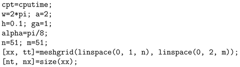
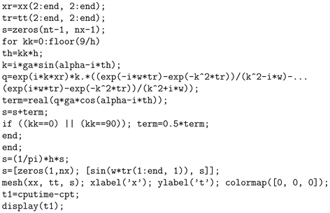
Appendix B. Code

For reference, this is the MATLAB/Octave code we used to compare the running times of Fokas’ method and our method and to generate FigureB1.

Figure B1. The solutions of the heat equation displayed on $x\in \left[\mathrm{0,1}\right]$ and $t\in \left[\mathrm{0,4}\pi \right]$ (left) and of Stokes equation displayed on $x\in \left[\mathrm{0,1}\right]$ and $t\in \left[\mathrm{0,1}\right]$ (right).

B.1. Our Matlab code for the heat equation

B.2. Flyer-Fokas’ code for the heat equation (Adapted from [3] )

Conflicts of Interest

The authors declare no conflicts of interest regarding the publication of this paper.

References

[1]	Fokas, A.S. (1997) A Unified Transform Method for Solving Linear and Certain Nonlinear PDEs. Proceedings of the Royal Society A, 453, 1411-1443. https://doi.org/10.1098/rspa.1997.0077
[2]	Fokas, A.S. (2002) A New Transform Method for Evolution PDEs. IMA Journal of Applied Mathematics, 67, 559-590. https://doi.org/10.1093/imamat/67.6.559
[3]	Flyer, N. and Fokas, A.S. (2008) A Hybrid Analytical-Numerical Method for Solving Evolution Partial Differential Equations in the Half-Line. Proceedings of the Royal Society A, 464, 1823-1849. https://doi.org/10.1098/rspa.2008.0041
[4]	Fokas, A.S., et al. (2009) A Semi-Analytical Numerical Method for Solving Evolution and Elliptic Partial Differential Equations. Journal of Computational and Applied Mathematics, 227, 59-74. https://doi.org/10.1016/j.cam.2008.07.036
[5]	Papatheodorou, T.S. and Kandili, A.N. (2009) Novel Numerical Techniques Based on Fokas Transforms for the Solution of Initial Boundary Value Problems. Journal of Computational and Applied Mathematics, 227, 75-82. https://doi.org/10.1016/j.cam.2008.07.031
[6]	Cody, W.J. (1969) Rational Chebyshev Approximations for the Error Function. Mathematics of Computation, 23, 631-637. https://doi.org/10.1090/S0025-5718-1969-0247736-4
[7]	Abramowitz, M. and Stegun, I. (1964) Handbook of Mathematical Functions. National Bureau of Standards, Applied Mathematics Series, 55.
[8]	Constantinides, E.D. and Marhefka, R.J. (1993) Efficient and Accurate Computation of the Incomplete Airy Functions. Radio Science, 28, 441-457. https://doi.org/10.1029/93RS00278
[9]	Levey, L. and Felsen, L.B. (1969) On Incomplete Airy Functions and Their Application to Diffraction Problems. Radio Science, 4, 959-969. https://doi.org/10.1029/RS004i010p00959
[10]	Michaeli, A. (1996) Asymptotic Analysis of Edge-Excited Currents on a Convex Face of a Perfectly Conducting Wedge under Overlapping Penumbra Region Conditions. IEEE Transactions on Antennas and Propagation, 44, 97-101. https://doi.org/10.1109/8.477533