Gravitational Waves in a Universe with Time-Varying Curvature

J. C. Botke

Nogales, Arizona, USA.

DOI: 10.4236/jhepgc.2021.72036                

Abstract

In this paper, we present a complete solution of Einstein’s equations for the gravitational wave (GW) problem. The full metric is taken in the usual way to be the sum of a background vacuum metric plus a perturbation metric describing the GW. The background metric used is characterized by time-varying curvature as described in a recent paper. The solution we develop here does exhibit some features found in the standard model but it also contains others that are not found in the standard model. One difference is that the solution with time-varying curvature only allows for outward-directed waves. While this might seem a minor point regarding the GW equations, it is actually a significant verification of the solution presented in our earlier paper. A more obvious difference is that the solution demands that the vacuum along with all matter must experience transverse motion with the passing of the waves. This fact leads to the idea that a new approach to the detection problem based on the Doppler effect could well be practical. Such an approach, if feasible, would be much simpler and less costly to implement than the large-scale interferometer system currently under development.

Keywords

Gravitational Waves, Time-Varying Curvature

1. Introduction

In a recent paper [1] , we proposed a new model of cosmology based on the idea that vacuum has content and serves as its own source. One consequence is that the curvature of spacetime must vary with time and these together require that the present-day scaling of the universe must be expanding exponentially. A number of predictions are made in that paper that agree with observation leading support to the idea that the model is correct. In this paper, we will examine the effect that time-varying curvature has on gravitational waves (GW) and for this reason, it would be useful to review at least Section 8 of our original paper for the background needed to understand some of the discussion presented here.

Because the present-day curvature is not large, one would not expect to see dramatic differences between the results found here and those of the standard model (see e.g. [2] ) but there are differences that are interesting. For one, with time-varying curvature, the equations only allow outgoing waves from the source. As will be explained in Section 5, this is in direct contrast to the situation with the standard model. In that case, the equations by themselves allow both outgoing and incomings waves to exist and it is a matter of choice to ignore the incoming waves. With time-varying curvature there is no choice; the dynamics must evolve in the direction of increasing entropy. Another consequence of the time variation is that the phase velocity of the waves is not exactly the speed of light. In other words, space exhibits an index of refraction that is not exactly unity. The most obvious difference, however, is that the complete solution demands that the vacuum and all ordinary matter must undergo transverse oscillations with the passing of the GW and this motion suggests the possibility of a new detection scheme based on the Doppler effect.

Here, we will be working with the full Einstein equations so our development is more rigorous than that of the standard model. The equations are fully constrained which makes it possible to determine both the magnitude of the GW metric and its functional dependence on parameters such as the angular velocity and size of the source.

As we just noted, things are moving. Because the wavelength of the GW is on the order of twice the Earth-Sun distance, on a terrestrial distance scale, any device such as an interferometer or, in fact, the entire Earth, is oscillating as a unit of fixed coordinate dimension and what an interferometer detects is the variation in the travel time of photons over a fixed coordinate distance due to the oscillating curvature. For much greater distances on the order of a half-wavelength, on the other hand, one also needs to account for the fact that, for example, the mirrors of a gigantic interferometer would be in relative motion. The travel time of a photon would then vary as a consequence of both the motion of the mirrors and the oscillation of the curvature along its path.

2. Model

Unlike the case with electromagnetic radiation, GW consists of oscillations of the already existing background curvature of spacetime so, in some ways, GW has more in common with water waves than with radiation. Because of the nonlinearity of the geometry, we cannot simply add a perturbation solution to the background solution but must instead deal with the full metric. We form the full metric in the usual way by adding a small perturbation metric to the background metric. The process of reducing the original equations to a set of linear equations for the perturbation components involves a sequence of steps that must be completed in the correct order. Starting with the full metric, we calculate the Riemann and Ricci tensors in the normal manner and, only afterward, do we simplify by dropping all terms but those with the 1^st order powers of the perturbation. This is not a trivial matter because it is essential that the action of GW is described in terms of the actual background metric with curvature rather than with an idealized flat metric.

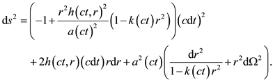
Unlike the standard model formulation which is based on a flat space metric, we are starting with the non-trivial background metric from [1] ,

(2-1)

Here, is the curvature and is the scaling, and the function is the off-diagonal coupling between the radial coordinate, r, and the time coordinate which is a necessary consequence of time-varying curvature. These have the values shown below,

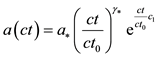, (2-2a)

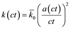, (2-2b)

, (2-2c)

and

(2-2d)

with the constants, , etc. all known.

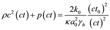
Another difference with respect to the standard model is that the background energy/momentum (EM) tensor is not zero. Again, from [1] , we have

. (2-3)

The background vacuum is at rest with the result that no velocities appear in this equation. The resulting Ricci tensor and the solution for the background metric components are given in the paper. (We note that with a flat metric, the Ricci tensor vanishes so in that case, Einstein’s equations for the background become just 0 = 0.)

The next step is to assume a form for the perturbation metric. The background metric is expressed in spherical coordinates and we considered formulating the analysis in those coordinates but it turned not to be convenient so we instead did this analysis in Cartesian coordinates. In the standard model in which the background is assumed to be a flat Minkowski space and with the vacuum described by, a number of simplifications are possible, such as making judicious use of gauge freedom to be simplified the model down to a simple wave equation. In our case, the non-vanishing energy-momentum tensor fixes the background vacuum which eliminates the possibility of any arbitrary simplifications. As a consequence, for our starting point, we assume a completely general symmetric metric and leave it entirely up to Einstein equations to determine the final form of the solution. Thus, where.

We now wish to calculate the Ricci tensor. We write where is the background metric and then compute the connection coefficients,

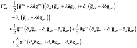(2-4)

The first term references only the coefficients of the background and the Ricci tensor that results will cancel against the background EM tensor. The perturbation coefficients are what remains,

(2-5)

We now need to consider just what is going on here. (Again, a review of Section 8 of [1] will make this more understandable.) First, we must remember that Einstein’s equations are local or, in other words, they are evaluated at a single point. From the point of view of the GW, at each point, (x, y, z), the wave experiences the background in the limit that the distance from that point vanishes. This means that if we take the immediate origin of our calculation to be that point, we should evaluate the background at that point, or in other words, we should set the background coordinates to zero. However, if we do so before calculating the Ricci tensor, we will lose all the curvature structure because the spatial derivatives do sample a region away from, albeit infinitesimally close to, the point. At the same time, we know that the background is the same everywhere so the spatial derivatives of the background in (2-5) must vanish. The time derivatives of the background, on the other hand, do not vanish because the background does depend on time. To actually develop and solve these equations, we used Mathematica^© Wolfram Research, Inc (and it would be impossible to complete the calculations by hand.) Accordingly, we needed to prevent the evaluation of spatial derivatives of the background. We accomplished this by replacing the spatial coordinates in the background metric with the coordinates. The background spatial derivatives in the connection coefficient calculation now vanish but the curvature structure is retained.

With the connection coefficients in hand, we next calculate the Ricci tensor and after doing so, because each point of the perturbation must experience the background evaluated at that point and because we have fixed our origin to be that point, we now set the background coordinates to. Finally, because the equations (but not the metric functions) must be independent of location (one point in the vacuum is exactly the same as any other point), the equations will be dependent on the spatial derivatives with respect to the coordinates but they cannot contain any explicit values of the coordinates (think of the standard wave equation) so we set those to zero which is again just evaluating the equations at the origin of each point.

The Riemann tensor is

(2-6)

and the Ricci tensor is then

. (2-7)

Turning now to the EM tensor, we have

(2-8)

where, , and are the vacuum energy density, pressure, and velocity variances induced by the passage of the GW. Expanding in the same way, we find

(2-9)

where is the background tensor. The perturbation tensor is then

(2-10)

where we have introduced the dimensionless velocity. The Einstein equations can be written in two ways and here, in keeping with the convention used in [1] , we will work with the EM trace reversed form so we have

. (2-11)

The final step is to include the source by combining its contribution with the vacuum EM tensor,. Lowering the indices of (2-9), trace reversing the result, and cancelling the background terms give us the final equations,

(2-12)

where is the source and S is its trace. The source tensor with be developed in detail in the next section.

In addition to these equations, we have the EM conservation condition,

(2-13)

which becomes after expansion

. (2-14)

Because the source is “over there”, it does not contribute to EM conservation at the location of the observer.

Also, because any small volume of the vacuum acts like ordinary matter under the influence of the curvature, we have an additional set of constraints given by the geodesic equations,

(2-15)

To first order in small values, the vacuum velocity has the following form

. (2-16)

Since the velocity is small, we can approximate and after changing the time coordinate to, we end up with,

(2-17)

In these equations, each chunk of the vacuum is concerned only with the connection coefficients at its location and first, because there are no spatial derivatives in (2-17) and second, because the background curvature is the same everywhere, we can immediately set. After doing so, we find that the only nonvanishing coefficients are. Writing out the equations gives us

. (2-18)

Since and, the time equation simplifies to

. (2-19)

At this point, we have 18 equations. It happens, however, that the two sets of equations, (2-14) and (2-18) are not all independent. After removing the redundant equations, we end up with a total of 14. Counting the variables, we have 10 metric components, , , and the 4 velocities for a total of 16. But and we will find that (2-19) implies that as far as the GW are concerned, , so we end up with a total of 14, the same as the number of equations.

With the equations now specified at least symbolically, we will turn to the source.

3. The Source

Because we are intending to find a complete solution for this problem, we must be explicit about the source and the choice we made was to consider a compact binary star system. The choice is, in fact, fairly general since most sources will involve an orbiting system of one sort or another. To keep things simple, we will consider a system of two stars of equal mass for which the frequency is

(3-1)

Here, M is the mass of each star and is the radius of the system. With stars of unequal mass, the formula of (3-1) would be modified but, since the final equations depend only on the angular frequency and the radius of the system, the choice of equal masses is not restrictive. From [3] , for compact binary systems such as pairs of white dwarfs or neutron stars typical baseline values are and which imply and. The wavelength is then. (For reference, the Earth-Sun distance is 1.49 × 10¹¹ m.) Because our time variable is with the dimensions of length, we define a corresponding scaled angular velocity which has the units of inverse length. Finally, the radius of the Milky Way is about 4.7 × 10²⁰ m which sets the scale for the Earth-source distance,.

We now chose to place the source at the point in the coordinate system. We also want to allow for an arbitrary orientation of the source so we introduce a second system obtained by a rotation about the shared axis. Figure 1 illustrates the two coordinate systems.

The stars orbit in the plane so their coordinates are

(3-2)

where the subscripts refer to each of the two stars. For the source EM tensor, however, we need the velocities in the system. A simple rotation gives

(3-3)

and taking derivatives with respect to gives us the velocities

(3-4)

We will approximate the stars as point objects so the density of the system becomes

(3-5)

Integrating this overall space gives

. (3-6)

Equation (3-5) gives the density in terms of an origin at the center of the rotating system. The observer, however, sees the system from a distance on the order of

Figure 1. Source coordinate systems.

and from the observer’s point of view, the offsets in the delta functions, which are of order, are extremely small and can safely be dropped. The z axis delta function, however, now becomes where z is measured relative to the observer’s coordinate system. From the point of view of the observer, the source is located at, i.e. the source density is zero everywhere except at. The density is then

. (3-7)

It is now a straight-forward matter to work out the components of the EM tensor. The complete tensor is the sum of the tensors for two stars with each adding a contribution of. Because their velocities are opposite, the contributions vanish. For all the other components, the contributions are equal and thus add

(3-8)

It now only remains to lower the indices and trace-reverse the result. The indices are lowered with the background metric so and the trace is. By expanding the sines and cosines, we see that the source has the form

(3-9)

where the tensors, , and are independent of time. In order to shorten the expressions a little, we introduced the shorthand, and. The non-vanishing components are listed in (3-10),

(3-10a)

(3-10b)

4. The Complete GW Equations

In this section, we will flesh out the symbolic equations presented above. It would require far too much space to present the entire development and, in any case, it is unlikely that anyone would be interested. Instead, we will outline the steps and present the full list at the end of the section. From this point on, everything was done with Mathematica so from here on out, we will use Mathematica’s notation¹.

In [1] , we found that physical quantities such as the curvature and the motion of particles are dependent only on the sum of the vacuum energy density and pressure rather than on either alone. Expecting a similar result here, the two quantities we worked with were that sum and again the pressure. The equations thus contain references to and instead of and. As it happens, the equations do not depend on just the sum but the influence of the energy density and pressure turns out to be very small.

The first steps were to convert the background metric, (2-1) to Cartesian coordinates and then to compute the inverse metric and the connection coefficients in the usual manner. After doing so, we made the change of names of the coordinates to the barred versions, , etc. We next expanded (2-3) in the usual manner to obtain the trace-reversed background EM tensor. Turning now to the perturbation metric, after expanding (2-6) and (2-7), we evaluate at each point (set and) to obtain the Ricci tensor, which is dependent on the 4 coordinates,.

We now want to apply some physical reasoning to simply this result. First, we know from [1] that signals travel along paths of constant angle and that the effect of the background curvature is entirely radial. We also know that any transverse interaction between elements of the gravitational wave would be 2^nd order in the metric components. Since the background vacuum is isotropic, to this level of approximation the anisotropy of the wave is entirely a result of the asymmetry of the source which we have expressed with the tilt angle. To get some idea of the magnitude of the velocity variance, we use the chain rule,. The derivative of any component with respect to is of the same order of magnitude as the component but the derivative introduces an additional factor of so the variance in the transverse directions is very small. We have oriented our coordinate system so the source lies on our z-axis and the smallness of the transverse variance then means that we can eliminate the x and y dependence from the equations.

In the far-field limit, the z coordinate differs from the radial distance to the source by an infinitesimal amount so we can also replace z with the radial distance, l. Finally, because the background metric functions vary slowly with time relative to the travel time from the source, we can evaluate them at the present-day time,. With these changes, we have reduced the problem to one with a single spatial dimension.

We next turn to the EM conservation equations, (2-14) and the vacuum geodesic equations, (2-18) and (2-19). We will spend a little more time on these because they are not all independent. After removing the transverse dependencies from (2-14), we obtain the following 4 equations. (From here on out, we will drop the bold font indicating a tensor, i.e. from now on.)

(4-1a)

(4-1b)

(4-1c)

(4-1d)

Doing the same with (2-18) gives us

(4-2a)

(4-2b)

(4-2c)

(4-2d)

The first of these states that does not vary with time which will eventually mean that does not contribute to the GW. Substituting the remaining equations into the EM equations eliminates (4-1b) and (4-1c). The remaining equations, (4-1a) and (4-1d) become

(4-3a)

. (4-3b)

The last equation states that the pressure does not vary with distance but this is the only place that the spatial derivative of the pressure appears in the equations so we can’t enforce this constraint by eliminating the derivative from the other equations. We will find from the final solution, however, that while this constrain is not satisfied exactly, the numerical value of the derivative is vanishingly small. The 8 equations we began with have now be reduced to 4; (4-3a) and (4-2b)-(4-2d).

We will now list the final equations. For brevity, we have omitted the arguments of the variables.

(4-4a)

(4-4b)

(4-4c)

(4-4d)

(4-4e)

(4-4f)

(4-4g)

(4-4h)

(4-4i)

(4-4j)

(4-4k)

(4-4l)

(4-4m)

. (4-4n)

The lower case in the first 10 equations is a place holder for the source and its value depends on which of the three sets of equations we are solving, , , or. Table 1 summarizes the dependences.

5. Solution of the GW Equations

Because this system of equations is now linear, we can use Fourier transforms (FT) to find the solution. We represent each variable by the general form

. (5-1)

Here, has the units of inverse length. It is now necessary to pin down the origin and it will be convenient to fix it at the source. In this case, the observer is now located at and the source is at so the argument of the z delta function is now just. The 3 delta functions in combine to become.

We will deal with the time variable first. We take the FT of both sides of the equations. On the LHS, we integrate by parts to replace the time derivatives with factors of and. The RHS has the form given by (3-9) and its FT is

(5-2)

The total solution is thus the sum of three partial solutions. The first with is static and hence does not contribute to the GW. The remaining two both contribute and because we are only interested in the inhomogeneous solution, we

Table 1. Summary of equation dependencies.

can set in the equations and in the equations. Earlier we saw that. In terms of its FT, this condition becomes so either or must vanish. In the static case, so will contribute but in the GW case, so as far as the GW equations are concerned.

Turning now to the spatial coordinates, we first replace the delta function in the source by its FT,

. (5-3)

After moving the source to the LHS, we end up with a list of equations with the symbolic form,

. (5-4)

Here, the subscript “j” is a shorthand for the indices taken in sequence. Since this must be true for all, the integrand in the parentheses must vanish which results in a system of equations for the. The is dependent only on the magnitude of the wave vector, , so the in turn are also only dependent on that magnitude.

After solving for the, the are calculated using

. (5-5)

The final solution is then. Because the only angle dependence in (5-5) is in the exponent, we can perform the angular integrations to obtain the one-dimensional form,

. (5-6)

when we solve the system of equations, we find that are even functions of k and since is also an even function, we can extend the lower limit of the integration to,

. (5-7)

The on the other hand, are odd functions of k so at first sight, it would appear that we can’t extend the lower limit. We can easily get around the problem, however, by defining an auxiliary function, even in k, such that the required metric function is given by the following derivative,

. (5-8)

With the integrations now over the entire real axis, we can employ contour integration to perform the final integrations. The have multiple simple poles that are shifted off the real axis by small amounts. We split the sine function into the sum,

(5-9)

which separates the integration into a sum of two integrals. For the first, we close the contour in the upper half-plane and in the second, in the lower half-plane.

At some point during the development of the solution, it becomes necessary to replace the symbolic parameters with numerical values. This, however, introduces a significant problem because of the vast range of magnitudes involved. For example, the scaling while a typical value of the angular frequency is. Also, and some of these appear in powers of up to 8. The issue is that with such a range of values, the order of combination is significant because of the limited precision of computers. For example, if we use the computer to evaluate, in that order the result will be zero whereas the correct result is 3. In this particular example, if we reorder the list to, the computer gives us the correct result and this is a strategy we sometimes used. Reordering was not always possible, however, so we developed other strategies to minimize the numerical errors. For example, we noticed that the combination appears often in the equations with n as large as 7. If we try replacing raised to the 7^th power and then multiply by to the 7^th power, we overflow the limits of the ability of the computer to represent numbers. The solution in this particular case is to multiply the two factors before raising to the power.

From Table 1, we see that appears alone in the single Equation (4-4f) and because this is the simplest case, we will walk through the steps to the solution. The others follow a similar pattern with variations. The final results are listed in Sec 7.

We first solve the FT version of (4-4f) with the source set to and find,

. (5-10)

In this case, the numerator is a constant so the integrand including the extra factor of k from (5-7) vanishes as. This is an even function of k that has the two poles,

. (5-11)

Putting in numbers, these become,

(5-12)

We now see one of the consequences of time-varying curvature. The poles are offset from the real axis by an amount proportional to which is entirely a consequence of time-varying curvature.

Because of the energy density and pressure, the real parts are not exactly but instead, have the values where. While this result is far too small to have any observational consequences, it does show that the vacuum exhibits an index of refraction that is not exactly unity and because the correction is negative, the phase velocity of the GW is slightly greater than c. This value was computed using the background vacuum properties far from any matter which of course is not the situation we are in. In [1] , we showed that the corresponding parameters in the interior of a galaxy can be expected to be perhaps 10⁷ times larger so the refraction offset will also be somewhat larger.

We now perform the contour integrations. The integral involving closes in the upper half-plane and captures the first pole thus becoming multiplied by a number very close to unity from the imaginary part. The integral involving closes in the lower half-plane. The real part of the pole is, in this case, negative which cancels the minus sign in the exponent. Also, its coefficient in (5-9) is −1 but because we are closing in the lower half-plane, there is another factor of −1 coming from the clockwise traverse of the contour. The net result is that the two contributions are the same. Because we are considering the contribution, this gets multiplied by so the result is an outgoing plane wave proportional to where n is the index of refraction.

The next step is to repeat the whole process for the source. It is apparent from (5-11) that reversing the sign of will change the signs of the imaginary parts of the two poles. This means that the integral now picks up a negative real part so the contribution is proportional to but this time, the time-dependent factor is so the result is which is again an outgoing wave. As before, the contribution is the same as the contribution.

The fact that the solution only allows for an outgoing wave is actually a significant result on more than one account. The standard model is based on a linearization of Einstein’s equations [2] that reduces to a simple wave equation, , which has a pair of poles on the real axis. Application of the Green’s function approach now requires that a choice be made as to how to offset the contours (see e.g. [4] ) to avoid the poles. One makes a choice based on one’s expectations regarding causality or some other criterion but that is still a choice. The equations don’t make the decision for you. There is nothing in the standard model, for instance, that would disallow a scenario in which inward bound waves could add energy to a binary system. With time-varying curvature, there is no choice; the equations make the decision. What this means is that the time-variance of the background curvature fixes the dynamics so that the entropy is always increasing. This result is a striking verification of the model presented in [1] . The direction of the offsets of the poles from the real axes are fixed by the sign of the metric function (2-2c). The solution of Einstein’s equations gives that function a positive value which we have seen implies outward bound waves. Had the solution returned a negative value, it would have implied inward bound waves and that would indeed have been a problem for the model.

We will now just outline the process for the remaining components. The FT solution for has a factor of k² in the numerator and a factor of k⁴ in the denominator so the integrand again vanishes as. The integrand is again an even function of k but this time there are two pairs of poles as indicated below,

(5-13)

The first pair is the same as for. The second set is a pair with a very small real value. This corresponds to a solution the varies with time but not with position (aside from the overall that arises from the spherical geometry.) A very small real value corresponds to an apparent index of refraction close to zero which in turn implies a phase velocity vastly larger than c. What we are seeing is a consequence of setting the transverse derivatives to zero. By doing so, we are in essence saying that the medium is infinitely stiff and such a medium would have an infinite phase velocity. This would also imply that the vacuum is acting on itself which we have disallowed from the very beginning. Of course, there is no such signal. The vacuum curvature is oscillating in synchrony without any transverse interaction at all at our level of approximation but from the point of view of the equations, the synchrony is a consequence of a very large phase velocity. It turns out in the end that the final contribution from these poles is extremely small and has no physical significance.

The solution for has the same structure as and, in fact, after dropping small values,.

The situation for is different again because it has a factor of k² in both its numerator and denominator and because of the extra factor of k in Equation (5-7), the integrand does not vanish as. In order to make the integral finite, we must introduce a cutoff. Large k corresponds to small distances so introducing a cutoff is equivalent to placing a limit on the minimum meaningful distance. A simple method that preserves the other desirable characteristics of the solution is to introduce another set of poles at (). These poles are on the imaginary axis far enough away from the real poles to not affect the solution. The poles this time have the values,

(5-14)

After completing the solution, we find that is proportional to which is zero by anyone’s reckoning. We only show this to illustrate the fantastic range of numbers that are involved in this business.

Next is. This component is an odd function of k so we introduce an auxiliary function which is even. The function vanishes as so the integration proceeds in the normal manner. In this case, the poles are,

(5-15)

Again, the real parts are very small and after the derivative in (5-8) is applied, the value of is reduced by another factor of 10⁻²⁰ so the result is that.

We now consider the energy density and pressure. Both and have the form k²/k² so again we need to add a cutoff. The poles for the pair are the same and are the same as those of. After doing the integrals and dropping small quantities, we find that and are equal. Since, we have the result,

(5-16)

It will not be immediately obvious, but in fact, is quite small. Remember that in the equations, gets multiplied by which greatly reduces its impact. A better comparison is with the background energy density. If we evaluate (5-16) with a value of, we find a magnitude of 10⁻¹⁷ kg·s⁻²·m⁻¹. The present-day background energy density, on the other hand, has a value at least as large as [1] so the perturbation is a factor of 10⁻⁷ smaller.

Referring back to the constraint of (4-3b), taking the derivative introduces an additional factor of so the numerical value of the constraint is indeed vanishingly small. The reason there is so little variation in the pressure and none at all in the energy density again goes back to the smallness of the transverse derivatives. Without any transverse variation, the vacuum is oscillating as a unit so there is no compression or expansion of the vacuum.

What remains now are the two sets of equations, (4-4b, g, and l) and (4-4c, i, and n).

6. Velocities

From (4-4l, m, n), we see that the velocities are given by, , and. The latter is easy. Because,. We next use the just named equations to eliminate the velocities from (4-4b) and (4-4c) which leaves us with two pairs of simultaneous equations. Taking the, pair first, solving for results in,

(6-1)

This has the expected pole structure which, in fact, it is the same as that of. When we solve for and, we find that but we also find that their magnitudes are wildly too large. The problem is the extremely small denominator in the second line of the equation so clearly, we need to make an adjustment. To get some idea of the magnitude, we set to zero in the FT of (4-4g) to obtain which suggests that a reasonable trial function is

. (6-2)

This, like (6-1), is an odd function of k so an auxiliary function will be required. After solving the equations, the derivative of (5-8) will cancel the factor of in the denominator. What we do next is to substitute this guess back into the equations and calculate the that results from each of the 2 equations separately. We then compute the final results and compare the values to see if the pair is consistent. The two are even functions of k with the same poles as but they are of the form k²/k² and so need a cutoff. After working through to the final solution, we find,

. (6-3)

Comparing the final two trial values of, we find that they are equal with a common value of,

(6-4)

We find again that so that seems to be a robust relationship.

Using the same procedure on the 2^nd set of equations, we find,

(6-5)

(6-6)

We see that these are 90˚ out of phase with each other. We also see that, aside from a factor of , these have the same magnitude and that this magnitude is consistent with the magnitudes of the other components.

It is important to appreciate that these results are solutions to the equations. While there is some uncertainty about the magnitude of the velocities, there is no uncertainty about the fact of the velocities because there is no solution of the equations with zero velocities. Another important point is that these results reflect the perturbation geodetic and so apply to all matter, not just the vacuum. The means, for example, that the entire Earth is undergoing transverse oscillations during the passing of a GW.

Clearly, something is missing from these equations which results in their being singular. The likely answer is that higher-order terms must be retained. In developing the equations, we made two assumptions. First, we assumed that we could linearize the equations with respect to the perturbation metric and second, we assumed that we could drop the transverse derivatives. The metric components are of and we learned earlier that the transverse derivatives are smaller so they are of. We might consider retaining just the transverse derivatives but the 2^nd order metric contributions would be of the same magnitude so if we retain one, it would be necessary to also include the other. These higher-order terms are probably not too important individually but including these would couple these equations to all the other equations. The first equation, for example, contains a term proportional to. The problem we then have is that including the higher-order terms would land us in an entirely new realm of difficulty. Instead of dealing with a 1-dimensional, linear problem, it would become necessary to solve a 3-dimensional, non-linear problem. At some point, it would be useful to explore the 3-dimensional problem but that would require far more computer capacity than we have available.

7. Summary and Detection

The complete solution is shown below.

(7-1a)

(7-1b)

(7-1c)

where

(7-1d)

Because of (3-1), only two of the parameters are independent. In summary, we have a solution that has some characteristics in common with the standard model, viz., and trace = 0. Unlike the case with the standard model, however, we arrived at these results by solving Einstein’s equations with a non-trivial background metric and a proper source energy/momentum tensor that is dependent on the velocities of the stars. These similarities are not imposed by making choices but instead are results obtained by solving the equations. The most notable difference is that this solution predicts values for the transverse velocities of the vacuum.

The final metric including the background is

(7-2)

We can simplify the results a little by recognizing that the argument, that appears in all the formulas is with respect to our chosen origin at the source. Shifting to a local origin amounts to just a phase shift. Next, because for any terrestrial detector, the variation in distance is extremely small compared to the wavelength of the GW, we can set. Thus, we can make the replacements,

(7-3)

We can now make a comparison with the standard model taking as an example, equation 18.19 of [2] . First, aside from a factor of, the magnitude of 18.19 is the same as. The signs of, , and appear to be different but that is just a matter of a phase change. Replacing by brings the solutions into agreement. The standard model solution corresponds to circularly polarized radiation with the same sense of rotation as the source. In this new solution, the magnitudes of and are not the same so the correspondence would be to elliptically polarization with again the same sense of rotation as the source. The solution here, however, is more complex because the metric contains additional components that couple the coordinates to both the time coordinate and the z coordinate. Everything still oscillates at the same frequency but not in a form that can be described as simple circular polarization. We also have the velocities. If we write

, (7-4)

we see that the motion is elliptical with axes, and but with a sense of rotation opposite that of the source.

We will now consider some implications for a detection system. First, we note that because the wavelengths of the GW are very large, everything on earth and, in fact, the earth itself undergoes the oscillation as a single unit. This follows from the fact that the geodetic is the same everywhere on Earth so that all terrestrial matter moves with the same velocity. We argued earlier that the transverse variance of the components is on the order of so the difference in the velocities of the two ends of a terrestrial interferometer would be on the order of 10⁻¹⁸ - 10⁻²⁰.

Consider for example, an arm oriented along the x-axis. For photons, , so we have,

. (7-5)

Because we are assuming the coordinate distance is very small, we can just solve this equation algebraically without needing to convert it into a differential equation. The result is,

(7-6)

Along the y-axis, we have

(7-7)

What the interferometer measures is the difference. For equal arm lengths, the result is,

. (7-8)

As noted earlier, if we consider some detection system on a much grander scale, we must account for the variation in the distance from some chosen origin in the arguments of the metric functions as well as the motions of both our chosen origin and the reflectors. Also, the metric must be treated as the definition of a set of differential equations, i.e., instead of we need to solve for, etc. and integrate over the appropriate paths.

8. Doppler Detection

The fact that distant sources would be in relative motion suggests that a detection system based on the Doppler effect might work. The idea would be to place a few satellites at distances on the order of 1/2 of the expected wavelength from the Earth and then to detect the Doppler frequency shift of signals returned from the satellites. The reason for that choice of distance is that it would maximize the relative GW velocity between the Earth and the satellite. The shift would be exceedingly small but the fact that its frequency would be known with considerable accuracy for any identified source should allow for the signal processing necessary to detect the GW.

We will set the stage with a few baseline numbers. The wavelength is given by so the nominal round-trip travel time with the satellite at a distance of ½ the wavelength would be T_s or about 16 mins. The corresponding frequency would be around 10⁻³ Hz. For a one-way trip, the frequency shift would be but because the satellite experiences a Doppler shift, the returned signal would have a shifted frequency which would be shifted again when received back on Earth so the round-trip frequency shift would be twice the value indicated. Given (7-1b), we would expect a shift on the order of 10⁻¹⁸ - 10⁻²⁰ depending on the distance to the source.

What seems to be the most sensible arrangement would be to generate a signal at a local base station that would be directed outwards toward the satellites that would then act as passive mirrors to send it back. To generate the signal, the outputs of one or more optical atomic clocks operating at a single frequency would be combined and then run through a frequency comb to generate a signal at an intermediate frequency suitable for transmitting. The Mars mission uses an X band (8 GHz) signal for communications so that might be a suitable choice because the large antennas needed already exist. The received signal would nominally be an image of the transmitted signal twice shifted in frequency by the Doppler effect or. We must also, however, account for the variation in the travel time of the signal as a result of the varying curvature along the path of the photons. This variation will retard or advance the time of arrival of each cycle of the signal so the effect would be to vary the phase of the received signal. The signal would then have the form,

(8-1)

Because of the extremely small frequency shift, it will be necessary to used interferometry in some form to detect the GW signal. If we heterodyned with a signal at the transmitted frequency, the output would be,

(8-2)

The first three terms have frequencies either at the transmitted frequency or at double that frequency and consequently are of no interest. The last term is the one that concerns us. Given that the transmitted frequency would likely be in the GHz range, the last term is a signal with an extremely low frequency (on the order of or 10⁻⁹ - 10⁻¹¹Hz) that is modulated at the frequency of the source,. Passing the output, (8-2), through a bandpass filter centered at the source frequency would leave us with a signal that would constitute detection of the GW. The additional phase term would also contribute at that frequency but its effect would be much smaller; on the order of rather than.

This scheme would have several advantages over an interferometric system if it can be made to work. For one, all the signal generation and processing would occur close to home. For another, the distance to the satellite only enters insofar that a distance of 1/2 wavelength would maximize the relative velocity. This means that the position would not need to be controlled or even known with any level of accuracy. The only significant constraint on a particular satellite would be the tilt angle dependencies of. Both of these vanish at, the velocity is maximal at and is maximal at. The only reason for positioning multiple satellites is that at least one or two should be in a favorable position for any particular source. A third advantage is that detection would only require the use of a single satellite so no coordination between multiple satellites would be necessary.

The concept seems to be feasible but, as is the case for any such scheme, noise will be the controlling factor. Optical atomic clocks at present have frequency uncertainties of at optical frequencies. Our primary concern, however, is with the noise levels at the GW frequency. Each step, all the way from the clocks to the satellite and back, is a potential noise source and all these would need to be analyzed by experts in the various disciplines to determine if this approach would work. As a final thought, we have no idea if it is even possible but if a continuous sampling of the transmitted signal could be stored for the duration of the transit time of the signal, it could be used as the reference signal in the heterodyning process in which case the noise would become part of the signal instead of being a problem.

9. Conclusion

In this paper, we have presented an analysis of GW in which the background metric is one with time-varying curvature. Some basic features of the standard model are found in the solution but the solution also contains other features that are not found in that model. Notably, the model predicts that both the vacuum and all matter must undergo oscillations with the passing of the GW, a result that leads to the idea of a detection system based on the Doppler effect. The model also predicts that only outbound GW is possible which stands as a significant verification of the time-varying curvature background model of [1] .

NOTES

¹The primary difference is the notion used for partial derivatives. Mathematica uses superscripts with functions of more than one variable, e.g. and primes for functions of a single variable, e.g..

^†Magnitude is uncertain. It could possibly be larger but probably not smaller.

Conflicts of Interest

The author declares no conflicts of interest regarding the publication of this paper.

References

[1]	Botke, J.C. (2020) A Different Cosmology: Thoughts from Outside the Box. Journal of High Energy Physics, Gravitation and Cosmology, 6, 473-566. https://doi.org/10.4236/jhepgc.2020.63037
[2]	Hobson, M.P., et al. (2006) General Relativity, An Introduction for Physicists. Cambridge University Press, Cambridge. https://doi.org/10.1017/CBO9780511790904
[3]	Wikipedia (2021) Gravitational Wave. https://en.wikipedia.org/wiki/Gravitational_wave
[4]	Green’s Function of the Wave Equation. http://ricardoheras.com/green-function-wave/