Physics-Aware Deep Learning on Multiphase Flow Problems

Zipeng Lin

Basis Independent Mclean, Mclean, USA.

DOI: 10.4236/cn.2021.131001                

Abstract

In this article, a physics aware deep learning model is introduced for multiphase flow problems. The deep learning model is shown to be capable of capturing complex physics phenomena such as saturation front, which is even challenging for numerical solvers due to the instability. We display the preciseness of the solution domain delivered by deep learning models and the low cost of deploying this model for complex physics problems, showing the versatile character of this method and bringing it to new areas. This will require more allocation points and more careful design of the deep learning model architectures and residual neural network can be a potential candidate.

Keywords

Deep Learning, Neural Network, Multi-Phase, Oil Incompressible, Fluid Physics, Partial Differential Equation

1. Introduction

Physics problems are usually expressed in a succinct way by partial differential equations (PDEs). The study of many physics phenomena and the forecast of physics dynamics require solving those expressed PDEs with the specified initial and boundary conditions. This procedure is conventionally conducted by implementing different numerical methods such as central difference in space dimension [1] and explicit/implicit Euler method [2] in time dimension. Those implementations, on one hand, are usually problems-centered and cannot be extended to other physics problems. On the other hand, the implementations need domain knowledge of numerical analysis to guarantee numerical stability and can be expensive to implement. Moreover, much commercial software for the numerical analysis of certain types of physics problems can be costly prohibitive for individual researchers and students.

The recent advance of deep learning technologies provides a potential alternative for researchers to obtain a quick understanding of the investigated physics problems. Those methods are developed to solve the PDES describing physics rules based on deep learning and avoid the need of numerical implementation. Those studies on the domains referred as physics informed neural network (PINN).

Khoo et al. [3] established a theoretical model for neural network to solve PDEs problems, which have uncertainties and used elliptic equations and nonlinear Schrödinger equations as examples considering a continuous-time dimension. Raissi et al. [4] incorporated PDEs residuals into the training objective of neural network and validated the methods on classic PDEs (including Burger’s equation and Navier-Stokes equation) with initial and boundary constraints. Bruton et al. [5] expanded the application of physics-informed neural network to fluid mechanics, and Kissas et al. [6] applied PINN to cardiovascular flows. Mauilk et al. [7] applied physics-informed machine learning to investigate problems concerning eddy-viscosity in fluid dynamics. All the works mentioned above focus on continuous time and space domains and fully connected neural networks are applied to surrogate the PDE solution.

Moreover, the theories of physics informed network have been extended on the discrete domains: Gao et al. [8] had extended the physics informed neural network to solve parametric PDEs on any irregular geometric domains; the Conservative Physics Informed Neural Network (CPINN) is invented to force nonlinear conservation laws on discrete domains by Jagtap et al. [9]; a parareal PINN, dividing a long time into parts of short time to solve the time-dependent PDEs more accurately to suit the physics problem into a coarse-grained solver, was introduced by Meng et al. [10]. Pang et al. have also extended the neural network into fractional PINN (fPINN) to solve inverse and forward questions when the data given is scattered.

In this study, we are particularly interested in investigating the applicability of PINNs on practical yet complex multi-phase flow problems. Despite the claimed success of PINNs on solving PDEs, the investigated PDES problems in existing literature are all simple, weakly coupled PDEs with relatively low nonlinearities. As far as we are concerned, no research has been conducted on the application of PINN for complex coupled flow problems.

In order to investigate the applicability of PINNs on practical yet complex multi-phase flow problems, the paper will proceed as follows. In Section 2, we present the model to the underground water physics problem, and how specifically our neural network model works. In Section 3, the general setup of the neural network, the data obtainment, and the process hyper-parameter tweaking. The results are presented in Section 3 and further insight and work in Section 4.

2. Methodology

2.1. Multi-Phase Flow Problems

In this study, we are interested in a multi-phase flow system. The study of multi-phase flow problems is an important key to understand the subsurface flow phenomenon that are common in aquifers, oil, and gas reservoirs, as well as many CO₂ sequestration fields. Specifically, here, we set up a two-phase oil water system described by two mass conservation equations:

$-\nabla \cdot \left({\rho }_o{u}_o\right)-q_o=\frac{\partial }{\partial t}\left(\phi {\rho }_o{S}_o\right)$ , for oil, (1)

And

$-\nabla \cdot \left({\rho }_w{u}_w\right)-q_w=\frac{\partial }{\partial t}\left(\phi {\rho }_w{S}_w\right)$ , for water, (2)

Here $\nabla$ is the Laplace operator which calculates the divergence of gradient, $\rho$ is the phase density, q is the source/sink term, $\phi$ is the rock porosity, S is the phase saturation which describes the proportion of the current phase in the porous media, and $u$ is the phase velocity respectively and can be computed by Darcy’s law:

$u_j=-\frac{k{k}_{rj}\left(S_j\right)}{{\mu }_j}\left(\nabla p_j-{\rho }_{j}g\nabla z\right),j=o,w$ (3)

where $k$ is the rock permeability that describes the rock capacity to transport fluids and $k_{rj}$ is the relative permeability that describes the additional capacity of the porous media to transport fluid with phase j, ${\mu }_j$ is the viscosity of phase j, $p_j$ is the pressure, and $\nabla z$ quantifies the depth change.

Pressure p and saturation S are the key variables that can describe the multi-phase flow dynamics and two extra equations are added here to conclude the mass conservation equations. First, the saturation of different phases ( $S_o$ represents the saturation of oil, $S_w$ represents the saturation of water) sums to be 1, i.e.,

$S_o+S_w=1$ (4)

and the pressure of different phases ( $p_o$ represents the pressure of oil, $p_w$ represents the pressure of water) is constrained by capillary pressure $P_c$ which can be usually assumed to be 0:

$p_o-p_w=P_c\approx 0$ (5)

Traditionally, the above mass conservation equations are closed by saturation and pressure constraints are solved by numerical methods on meshed grids. In this study, we will investigate the deep learning methods for the above two-phase flow problems in a one-dimensional scenario.

2.2. Deep Learning Models

Machine learning has had a splendid leap in the past few years, while deep learning, a sub-field of machine learning, has gradually reformed and enhanced the study of many research areas, including natural language processing and computer vision [11], image reconstruction [12], recognition [13] and general processing [14]. In this section, we explain the principals behind the deep learning technique from a higher, general level.

In a neural network, there are many neuron layers with neurons filled on each layer. The nonlinear activation functions applied on the matrix computation between adjacent layers result in a good approximation of complex nonlinear functions after combination of many connected layers. The Fully Connected Network (FCN), also named as multi-layer perceptron (MLP), is the most prominent architecture of this kind. Figure 1 is exemplary of the standard FCN architecture. Specifically, Figure 1 shows that Self-Made Neural Network Diagram has one hidden layer, one input layer and one output layer. Inside the FCN, the parameters used are the matrix weights defining the new relationship between two adjacent layers by the activation function. The output of the neuron of the former layer becomes the input of the neuron on the next layer. In all, the recursive function can be expressed by:

$x_{l+1}=f\left(W_l^{\text{T}}{x}_l+b_l\right)$ , (6)

where $x_l$ is the neuron values and $b_l$ is the bias at layer l, and f is the nonlinear activation function. There are many activation functions, the most prominent of which are sigmoid [15], tanh [16] and Relu [17].

On the low level of the mechanics of FCN, the weights are calculated using a loss function (a metric quantifying the difference between the target data and the neural network’s output) and back propagation. In this process, the lost function is minimized using an optimizer: a stochastic mini-batch gradient decent [18] and its variants such as RMSProp [19].

2.3. PDE-Aware Deep Learning

The core idea of utilizing deep learning on approximating PDE solutions is formulating the PDE residuals, as well as the initial and boundary conditions as the training loss. The objective of training deep neural network models is minimizing the defined loss by back-propagation [20]. To approximate the PDE solution of the studied two-phase problem, we construct a fully connected neural network (FCN) described in Section 2.2. The input of this FCN is the variable at space dimension x and time dimension t, the output of the neural network is the primary variables pressure p and saturation S, which are the solutions of the PDEs. The high-level implementation python code using tensorflow package [21] is presented. (Code Block 1)

Figure 1. Self-made neural network diagram.

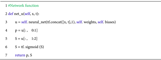
Code Block 1. Neural network.

Furthermore, to guide the constructed FCN to learn solving the target PDEs, the PDEs, along with its initial and boundary conditions, is reformulated in the residual form and treated as the training loss. The derivative terms in the PDE formulations are approximated by the gradient of the FCN output (p and S) with respect to the FCN input (x and t) and are computed by chain rule. We consider incompressible (fluid density is not a function of pressure) two phase flows and assume that the capillary pressure is 0. We also consider highly nonlinear problems with relative permeability defined as a nonlinear function of water saturation S_w. Viscosities of both oil and water are constant, and the absolute permeability k is assumed to be constant in this case. The code block below describes the formulation of PDE residuals using tensorflow, where “residuals” defines the two PDE residuals for mass conservation equations of two phase fluid (Equations (1) and (2)). (Code Block 2)

And the training objective will be the combination of three loss terms: mass conservation residuals, initial condition loss and boundary condition loss. The implementation of those losses can be as simple as what is shown in the code chunk. (Code Block 3)

3. Experiment Setup

In this section, we describe the detailed problem we are solving, data retrieving and model setup.

3.1. Physics Problem

The specific problem studied here is a water displacing oil problem in a one-dimensional tube filled with oil in the initial state, where water is injected from the left side of the tube to displace oil out of the tube, due to the immiscibility of those two phases.

As shown in Figure 2, water phase is injecting from the left end of the tube (colored by blue in the figure), while oil phase is displaced from the tube (colored by red in the figure). The Neumann boundary conditions are imposed at left and right boundaries, i.e., the inlet and outlet pressure gradients are constrained and set to be constant. Here, the normalized pressure gradient at both inlet and outlet boundaries are −2. Meanwhile, the injected water saturation is

Code Block 2. Neural network for PDE residual.

Code Block 3. Loss function.

Figure 2. Problem setup illustration. Water phase is injected from the inlet to displace the oil phase in the tube.

0.6, meaning water fraction is 60% while oil fraction is 40% in the injected water phase, and the water saturation in the oil phase is 0.3, meaning that water fraction is 30% and oil fraction is 70% in the oil phase. Furthermore, we assume that the tube is filled up with oil phase, meaning that the initial water saturation in the tube is 0.3.

With Equations (1)-(3), the relative permeability of different phases is the square of the corresponding saturation. More implementation’s details can be referred to code block 2.

3.2. Data Preparation

To prepare the data for the introduced deep learning model, we generate the data on the initial and boundary conditions as well as allocation points, which are the meshed data points in the domain of space and time. The one-dimension space and time are meshed with 500 and 200 grids respectively and therefore, we have 500 × 200 = 100,000 allocation points in total. Only the mass balance equation loss is enforced on those allocation points, meaning that the solved pressure and saturation should follow the mass balance equations at any of those allocation points. Meanwhile, on the boundary (space) locations and initial time, the solved pressure and saturation should also follow those constraints. It is worth noting that except for boundary and initial conditions where pressure (or the pressure gradient) and saturation have to follow the specified values, all the data are essentially just meshed grids over the space and time domain.

3.3. Solution Domain

The model takes about 200 seconds to converge on a single K80 GPU for this 1D problem with 100,000 allocation points. The solution domain is presented in Figure 3. As illustrated, the inlet is at x = 0 and outlet is at x = 500. The initial time is at t = 0 and the end time is at t = 200. Initially, the tube is filled with oil phase whose water saturation is 0.3, and therefore, the horizontal “line” at t = 0 is entirely colored dark blue. As time goes by, more water phase enters the tube and displaces the oil phase in the original tube. This phenomenon is reflected in Figure 3: as t increases from 0 to 200, the water phase colored by yellow gradually occupies the tube. The interface between the yellow and dark blue color in Figure 3 reflects the two phase interface. The immiscible property of two phases forms this interface, which is named “shock” in physics, is captured by the deep learning model. “Shock” in physics is noncontiguous, while the continuous deep learning model is able to capture this shock by approximating the discontinuity by sharp continuous changes.

Meanwhile, the pressure domain solution is displayed in Figure 4, where the color denotes the normalized pressure distribution. Remember we have Neumann boundary conditions, i.e. constant pressure gradient at the inlet and outlet boundaries, and therefore the pressure at boundaries is derived from the solution. Furthermore, unlike the saturation governed by hyperbolic equation, where the shock can be formed, the pressure is described by elliptic equation and therefore, the overall pressure solution field is continuous. The pressure in the inlet has to increase along with time to maintain the inlet pressure gradient, and so is the outlet pressure, which is captured by the deep learning solution as well.

3.4. Shock Propagation

In Figure 5, we present the visualization of front water saturation at different space locations at different time. This water saturation shock wave will march forward as water phase is kept injecting from the inlet of the tube. It can be observed that the overall shock march is captured by the deep learning model, as the vertical line describes correctly the saturation shock concept. However, it is also evident that the deep learning model smooths the transition a little bit, which is due to the fundamental continuity of deep learning models. This can be further solved by introducing nonlinear activation functions with sharper transition properties such as sigmoid in the last few deep learning model layers.

Figure 3. Saturation field solution in space x and time t. The color denotes the water saturation. The left side of the interface is the water phase and the right side of the interface is the oil phase. This interface denotes the “shock” in physics and is captured by the deep learning model.

Figure 4. Pressure field solution in space x and time t. The color denotes the normalized pressure distribution.

Figure 5. Water saturation front at different space locations.

4. Conclusions

In this study, we introduce the PDE is aware deep learning models for complex coupled multiphase flow problems. The fundamentals are formulating the governing PDEs, as well as initial and boundary conditions, into the training objective of the deep learning models, which can guide the deep learning models to find the physics pattern behind the governing PDEs and deliver the PDE solution over the interesting domain. The introduced deep learning model is a fully connected neural network with input as the PDE variables such as space x and time t and output such as the PDE solution at that specific x and t. In this way, the trained PDE aware deep learning model can effectively solve the coupled PDEs and deliver reasonable solutions. The PDE aware deep learning model provides an effective method for researchers in various physics field to quickly evaluate PDE solutions of the problems that they are interested in without the need to access expensive numerical solvers, which can be a potential and useful tool to fill the gap between expensive commercial software tools and research groups with limited funding.

For future work, we will consider more complex multiphase problems with compressible fluid and extend it to 2D space domains. This will require more allocation points and more careful design of the deep learning model architectures and residual neural network can be a potential candidate. Moreover, it will also be interesting to combine with physics experiment data to invert the solid and fluid properties in the multiphase flow governing equations.

Acknowledgements

After learning differential equations and realizing that some of the equations couldn’t be solved numerically while the solution pattern is random, I started to think of a way to solve those equations in a common way. Later reading the papers on this topic and more about neural network, I learned the idea of using neural network and then applied it to a problem that no one had applied before.

I want to thank my school math and physics teacher Dr. Ryan Grove, who introduced me to the thoughts of deep learning and provided me a chance to study python library such as matplotlib and numpy, which are crucial in my research. He also guided me through differential equations in math class and encourages me to code solutions for unsolvable equations. In research paper, he advised me and proofread my research paper, which is entirely written on my own.

The open-sourced python libraries, such as numpy and matplotlib, are also crucial to this project. I want to thank all the contributors and the community, which not only provide substantial help to coders and also showed me the importance of community and collaboration, and also the open spirit of geek to help the world generously.

I also want to express my gratitude to the Yau High School Science Award which provides me a chance to discover my interested topics. My biggest interest is math, physics and computer science, where I learned who to view this world rationally and solved interesting problems. When learning the Laplace transform in differential equation and the concept of convectional neural network, I was fascinated by those works of art by scientists and resolve to do such contribution, starting from doing research here. When seeing the beautiful equations in AP Physics C mechanics, such as the linear momentum and also the circuits ones in AP Physics Electricity and Magnetism, I realized the beauty of this world and wanted to solve those equations.

Finally, it is never enough to fully express my thanks and love to my teacher Dr. Grove and my parents, who supported me on this route of discovery!

Conflicts of Interest

The author declares no conflicts of interest regarding the publication of this paper.

References

[1]	Moore, P.K. (1999) Finite Difference Methods and Spatial a Posteriori Error Estimates for Solving Parabolic Equations in Three Space Dimensions on Grids with Irregular Nodes. SIAM Journal on Numerical Analysis, 36, 1044-1064. https://doi.org/10.1137/S0036142997322072
[2]	Burrage, K. and Tian, T.H. (2001) The Composite Euler Method for Stiff Stochastic Differential Equations. Journal of Computational and Applied Mathematics, 131, 407-426. https://doi.org/10.1016/S0377-0427(00)00259-4
[3]	Khoo, Y., Lu, J.F. and Ying, L.X. (2017) Solving Parametric PDE Problems with Artificial Neural Networks.
[4]	Raissi, M., Perdikaris, P. and Karniadakis, G.E. (2019) Physics-Informed Neural Networks: A Deep Learning Framework for Solving Forward and Inverse Problems Involving Nonlinear Partial Differential Equations. Journal of Computational Physics, 378, 686-707. https://doi.org/10.1016/j.jcp.2018.10.045
[5]	Brunton, S.L., Noack, B.R. and Koumoutsakos, P. (2020) Machine Learning for Fluid Mechanics. Annual Review of Fluid Mechanics, 52, 477-508. https://doi.org/10.1146/annurev-fluid-010719-060214
[6]	Kissas, G., et al. (2020) Machine Learning in Cardiovascular Flows Modeling: Predicting Arterial Blood Pressure from Non-Invasive 4D Flow MRI Data Using Physics-Informed Neural Networks. Computer Methods in Applied Mechanics and Engineering, 358, Article ID: 112623. https://doi.org/10.1016/j.cma.2019.112623
[7]	Maulik, R., et al. (2018) Data-Driven Deconvolution for Large Eddy Simulations of Kraichnan Turbulence. Physics of Fluids, 30, Article ID: 125109. https://doi.org/10.1063/1.5079582
[8]	Gao, H., Sun, L.N. and Wang, J.-X. (2020) PhyGeoNet: Physics-Informed Geometry-Adaptive Convolutional Neural Networks for Solving Parametric PDEs on Irregular Domain.
[9]	Jagtap, A.D., Kharazmi, E. and Karniadakis, G.E. (2020) Conservative Physics-Informed Neural Networks on Discrete Domains for Conservation Laws: Applications to Forward and Inverse Problems. Computer Methods in Applied Mechanics and Engineering, 365, Article ID: 113028. https://doi.org/10.1016/j.cma.2020.113028
[10]	Meng, X.H., et al. (2020) PPINN: Parareal Physics-Informed Neural Network for Time-Dependent PDEs. Computer Methods in Applied Mechanics and Engineering, 370, Article ID: 113250. https://doi.org/10.1016/j.cma.2020.113250
[11]	Guo, J., et al. (2020) GluonCV and GluonNLP: Deep Learning in Computer Vision and Natural Language Processing. Journal of Machine Learning Research, 21, 1-7.
[12]	Belthangady, C. and Royer, L.A. (2019) Applications, Promises, and Pitfalls of Deep Learning for Fluorescence Image Reconstruction. Nature Methods, 16, 1215-1225. https://doi.org/10.20944/preprints201812.0137.v2
[13]	Liu, C., et al. (2016) Deepfood: Deep Learning-Based Food Image Recognition for Computer-Aided Dietary Assessment. In: International Conference on Smart Homes and Health Telematics, Springer, Berlin, 37-48. https://doi.org/10.1007/978-3-319-39601-9_4
[14]	Perez, L. and Wang, J. (2017) The Effectiveness of Data Augmentation in Image Classification Using Deep Learning.
[15]	Mourgias-Alexandris, G., et al. (2019) An All-Optical Neuron with Sigmoid Activation Function. Optics Express, 27, 9620-9630. https://doi.org/10.1364/OE.27.009620
[16]	Abdelouahab, K., Pelcat, M. and Berry, F. (2017) Why TanH Is a Hardware Friendly Activation Function for CNNs. Proceedings of the 11th International Conference on Distributed Smart Cameras, Stanford, 5-7 September 2017, 199-201. https://doi.org/10.1145/3131885.3131937
[17]	Agarap, A.F. (2018) Deep Learning Using Rectified Linear Units (relu).
[18]	Li, M., et al. (2014) Efficient Mini-Batch Training for Stochastic Optimization. Proceedings of the 20th ACM SIGKDD International Conference on Knowledge Discovery and Data Mining, New York, 24-27 August 2014, 661-670. https://doi.org/10.1145/2623330.2623612
[19]	Bengio, Y. and Ca, M. (2015) Rmsprop and Equilibrated Adaptive Learning Rates for Nonconvex Optimization.
[20]	Gent, C.R. and Sheppard, C.P. (1992) Special Feature. Predicting Time Series by a Fully Connected Neural Network Trained by Back Propagation. Computing & Control Engineering Journal, 3, 109-112. https://doi.org/10.1049/cce:19920031
[21]	Abadi, M., et al. (2016) TensorFlow: A System for Large-Scale Machine Learning. 12th Symposium on Operating Systems Design and Implementation, Savannah, 2-4 November 2016, 265-283.