Numerical Solution of Fractional Differential Equations

Adnan Daraghmeh^*, Naji Qatanani, Aya Saadeh

Department of Mathematics, Faculty of Science, An-Najah National University, Nablus, Palestine.

DOI: 10.4236/am.2020.1111074                

Abstract

In this article, two numerical techniques, namely, the homotopy perturbation and the matrix approach methods have been proposed and implemented to obtain an approximate solution of the linear fractional differential equation. To test the effectiveness of these methods, two numerical examples with known exact solution are illustrated. Numerical experiments show that the accuracy of these methods is in a good agreement with the exact solution. However, a comparison between these methods shows that the matrix approach method provides more accurate results.

Keywords

Fractional Calculus, Fractional Differential Equations, Homotopy Perturbation Method, Matrix Approach Method

1. Introduction

Fractional differential equations appear frequently in various fields involving science and engineering, namely, in signal processing, control theory, diffusion, thermodynamics, biophysics, blood flow phenomena, rheology, electrodynamics, electrochemistry, electromagnetism, continuum and statistical mechanics and dynamical systems. For more details on the applications of fractional differential Equations (see [1] [2] [3] [4] [5] ). The concept of fractional calculus is now considered as a partial technique in many branches of science including physics (Oldham and Spanier [6] ). Srivastava et al. [7] gave the model of under actuated mechanical system with fractional order derivative and Sharma [8] studied advanced generalized fractional kinetic equation in Astrophysics. Caputo [9] reformulated the more “classic” definition of the Riemann-Liouville fractional derivatives in order to use integer order initial conditions to solve his fractional order differential equation. Kowankar and Gangel [10] reformulated the Riemann-Liouville fractional derivative in order to differentiate nowhere differentiable fractal functions.

In general, most of fractional differential equations do not have exact solutions. Instead, analytical and numerical methods become increasingly important for finding solution of fractional differential equations. In recent years, many efficient methods for solving FDEs have been developed. Among these methods are the monotone iterative technique [11] [12], topological degree theory [13], and fixed point theorems [14] [15] [16]. Moreover, numerical solutions are obtained by the following methods: the Adomian decomposition method and the variational iteration method [17], homotopy perturbation method [18] [19], Haar wavelet operational method [20], Neural networks [21], and so forth. Very recently, Hamdan et al. [22] applied Haar Wavelet and the product integration methods to solve the fractional Volterra integral equation of the second kind. In addition, Saadeh [23] in her master thesis has employed several numerical methods for solving fractional differential equations. These methods are the Adomian decomposition method, Homotopy perturbation method, Variational iteration method and Matrix approach method. A comparison between these methods has been carried out. In spirit, our numerical methods, namely the homotopy perturbation and the matrix approach methods are an improvement to those methods presented in the master thesis by one of the authors of this article. A comparison between these methods is carried out by solving some test examples using MAPLE software.

The paper is organized as follows: In Section (2) we recall some basic definitions and notions concerning fractional calculus. In Section (3), we introduce the homotopy perturbation method. The matrix approach method is addressed in Section (4). The proposed methods are implemented using numerical examples with known analytical solution by applying MAPLE software in Section (5). Conclusions are given in Section (6).

2. Mathematical Preliminaries and Notions

In this section, we review some necessary definitions and mathematical preliminaries concerning fractional calculus that will be used in this work.

Definition 1. [24] The Riemann-Liouville fractional integral operator of order $p>0$, $m-1<p\le m$, $m\in \mathbb{N}$ of a function $u\left(x\right)$ is defined as

$j^{p}u\left(x\right)=\frac{1}{\Gamma \left(p\right)}{\displaystyle \underset{0}{\overset{x}{\int }}}{\left(x-t\right)}^{p-1}u\left(t\right)\text{d}t,x>0$

Definition 2. [25]: (Riemann-Liouville Derivative): Let $n-1<p<n\in {\mathbb{Z}}^{+}$. The Riemann-Liouville derivative of fractional order p is defined as:

$D_{0,t}^{p}u\left(t\right)=\frac{1}{\Gamma \left(n-p\right)}\frac{{\text{d}}^n}{\text{d}{t}^n}{\displaystyle \underset{0}{\overset{t}{\int }}}\frac{u\left(\tau \right)}{{\left(t-\tau \right)}^{p+1-n}}\text{d}\tau$ (1)

Definition 3. [26]: The Grumwald-Letnikov fractional derivative with fractional order p if $u\left(t\right)\in {ℂ}^n\left[\mathrm{0,}t\right]$, is defined as:

${}_{a}D{}_t^{p}u\left(t\right)=\underset{\begin{array}{c}h\to 0\\ mh=t-a\end{array}}{\lim }{h}^{-p}{\displaystyle \underset{i=0}{\overset{m}{\sum }}}{\left(-1\right)}^i\left(\begin{array}{c}p\\ i\end{array}\right)u\left(t-ih\right)$ (2)

where $\left(\begin{array}{c}p\\ i\end{array}\right)=\frac{\Gamma \left(p+1\right)}{i!\left(\Gamma \left(p+1\right)\right)}$.

Definition 4. [6]: Grunwald-Letnikov fractional derivative of the power function $g\left(t\right)={\left(t-c\right)}^p$ is given as:

${}_{c}D{}_t^{\alpha }{\left(t-c\right)}^p=\frac{\Gamma \left(p+1\right)}{\Gamma \left(-\alpha +p+1\right)}{\left(t-c\right)}^{p-\alpha }$ (3)

Definition 5. [27]: The Caputo derivative of fractional order p of a function $u\left(t\right)$ is defined as

$D_{\ast }^{p}u\left(t\right)=\{\begin{array}{ll}\frac{1}{\Gamma \left(n-\alpha \right)}{\displaystyle \underset{0}{\overset{t}{\int }}}\frac{u^n\left(\tau \right)}{{\left(t-\tau \right)}^{\alpha +1-n}}\text{d}\tau ,\hfill & n-1<\alpha <n\hfill \\ \frac{{\text{d}}^{n}u\left(\tau \right)}{\text{d}{t}^n},\hfill & \alpha =n\in \mathbb{N}\hfill \end{array}$ (4)

Theorem 1. [28]: The Caputo fractional derivative of the power function satisfies:

$D_{\ast }^{\alpha }{t}^c=\{\begin{array}{ll}\frac{\Gamma \left(c+1\right)}{\Gamma \left(c-\alpha +1\right)}{t}^{c-\alpha }=D^{\alpha }{t}^c,\hfill & n-1<\alpha <n,c>n-1,c\in ℝ\hfill \\ 0,\hfill & n-1<\alpha <n,c\le n-1,c\in \mathbb{N}\hfill \end{array}$ (5)

Theorem 2. [26]: Leibniz rule for Riemann-Liouville fractional derivative: Let $t>0$, $\alpha \in ℝ$, $m>\alpha >m-1$, and $m\in \mathbb{N}$. If $u\left(t\right)\mathrm{,}g\left(t\right)$, and their derivatives are continuous on $\left[\mathrm{0,}t\right]$, then the following holds:

$D^{\alpha }\left(u\left(t\right)g\left(t\right)\right)={\displaystyle \underset{k=0}{\overset{\infty }{\sum }}}\left(\begin{array}{c}\alpha \\ k\end{array}\right)\left[D^{k}g\left(t\right)\right]\left[D^{\alpha -k}u\left(t\right)\right]$ (6)

Proof. See [26] for more details.

Theorem 3. [29]: Leibniz rule for Caputo fractional derivative: Let $t>0$, $p\in ℝ$, $m>p>m-1$, and $m\in \mathbb{N}$. If $u\left(t\right)\mathrm{,}g\left(t\right)$, and their derivatives are continuous on $\left[\mathrm{0,}t\right]$, then the following holds

$D_{\ast }^p\left(u\left(t\right)g\left(t\right)\right)={\displaystyle \underset{i=0}{\overset{\infty }{\sum }}}\left(\begin{array}{c}p\\ i\end{array}\right)\left[D_{\ast }^{p}g\left(t\right)\right]\left[D_{\ast }^{p-i}u\left(t\right)\right]-{\displaystyle \underset{i=0}{\overset{m-1}{\sum }}}\frac{t^{i-p}}{\Gamma \left(i+1-p\right)}{\left(u\left(t\right)g\left(t\right)\right)}^{\left(i\right)}$ (7)

Proof. See [29] for more details.

3. Homotopy Perturbation Method (HPM)

The fractional initial value problem in the operator form is:

$D^{\alpha }f\left(t\right)+Lf\left(t\right)=g\left(t\right)$ (8)

$f^{\left(i\right)}\left(0\right)=c_i,i=0,1,2,\cdots ,n-1$ (9)

where $c_i$ is the initial conditions, L is the linear operator which might include other fractional derivative operators $D^{\beta }\left(\beta <\alpha \right)$, while the function g, the source function is assumed to be in $c_{-1}$ if $\alpha$ is an integer, and in $c_{-1}^1$ if $\alpha$ is not an integer. The solution $f\left(t\right)$ is to be determined in $c_{-1}^n$.

In virtue of [16], we can write Equation (8) in the homotopy form

$\left(1-p\right)D^{\alpha }f+p\left[D^{\alpha }f+Lf\left(t\right)-g\left(t\right)\right]=0$ (10)

or

$D^{\alpha }f+p\left[Lf\left(t\right)-g\left(t\right)\right]=0$ (11)

where $p\in \left[\mathrm{0,1}\right]$ is an embedding parameter. If $p=0$, Equations (10) and (11) become

$D^{\alpha }f=0$ (12)

when $p=1$, both Equations (10) and (11) yields the original FDE Equation (8).

The solution of Equation (8) is:

$f\left(t\right)=f_0\left(t\right)+p{f}_1\left(t\right)+p^2{f}_2\left(t\right)+p^3{f}_3\left(t\right)+\cdots$ (13)

Substituting $p=1$ in Equation (13) then we get the solution of Equation (8) in the form:

$f\left(t\right)=f_0\left(t\right)+f_1\left(t\right)+f_2\left(t\right)+f_3\left(t\right)+\cdots$ (14)

Substituting Equation (13) into Equation (11) and collecting all the terms with the same powers of p, we get:

$p^0:D^{\alpha }{f}_0=0$ (15)

$p^1:D^{\alpha }{f}_1=-L{f}_0+g\left(t\right)$ (16)

$p^2:D^{\alpha }{f}_2=-L{f}_1\left(t\right)$ (17)

$p^3:D^{\alpha }{f}_3=-L{f}_2\left(t\right)$ (18)

and so on.

Following [6], we can write the first three terms of the homotopy perturbation method solution as:

$f_0={\displaystyle \underset{i=0}{\overset{n-1}{\sum }}}{f}^{\left(i\right)}\left(0\right)\frac{t^i}{i!}={\displaystyle \underset{i=0}{\overset{n-1}{\sum }}}{c}_i\frac{t^i}{i!}$

$f_1=-{\Omega }^{\alpha }\left[L{f}_0\left(t\right)\right]+{\Omega }^{\alpha }\left[Lg\left(t\right)\right]$

$f_2=-{\Omega }^{\alpha }\left[L{f}_1\left(t\right)\right]$

$f_3=-{\Omega }^{\alpha }\left[L{f}_2\left(t\right)\right]$

The general form of the HPM solution is:

$f_n=-{\Omega }^{\alpha }\left[L{f}_{n-1}\left(t\right)\right]$

The homotopy perturbation solution takes the general form:

$f\left(t\right)=f_0+f_1+f_2+f_3+\cdots +f_n+\cdots$ (19)

4. Matrix Approach Method

4.1. Left-Sided Fractional Derivative

Consider a function $g\left(x\right)$, defined in $\left[c\mathrm{,}d\right]$, such that $g\left(x\right)\equiv 0$ for $x<c$ and of real order $m-1\le \alpha \le m$, such as:

${}_{c}D{}_x^{\alpha }g\left(x\right)=\frac{1}{\Gamma \left(m-\alpha \right)}{\left(\frac{\text{d}}{\text{d}x}\right)}^m{\displaystyle \underset{c}{\overset{x}{\int }}}\frac{g\left(ϵ\right)\text{d}ϵ}{{\left(x-ϵ\right)}^{\alpha -m+1}},\left(c<x<d\right)$ (20)

Let us take equidistant nodes with the step size

$l:x_i=il\left(i=0,1,\cdots ,N\right)$

in the interval $\left[c\mathrm{,}d\right]$, where $x_0=c$ and $x_N=d$. Using the backward fractional difference approximation for the derivative at the points $x_i,i=0,1,\cdots ,N$, we have:

${}_c{D}_{x_i}^{\alpha }g\left(x\right)\approx \frac{{\nabla }^{\alpha }g\left(x_i\right)}{l^{\alpha }}=l^{-\alpha }{\displaystyle \underset{j=0}{\overset{i}{\sum }}}{\left(-1\right)}^j\left(\begin{array}{c}\alpha \\ j\end{array}\right)g_{i-j},i=0,1,2,\cdots ,N$ (21)

Equation (21) is equivalent to the following matrix form [11]:

$\left(\begin{array}{c}{l}^{-\alpha }{\nabla }^{\alpha }g\left(x_0\right)\\ l^{-\alpha }{\nabla }^{\alpha }g\left(x_1\right)\\ l^{-\alpha }{\nabla }^{\alpha }g\left(x_2\right)\\ ⋮\\ l^{-\alpha }{\nabla }^{\alpha }g\left(x_{N-1}\right)\\ l^{-\alpha }{\nabla }^{\alpha }g\left(x_N\right)\end{array}\right)=\frac{1}{l^{\alpha }}\left(\begin{array}{cccccc}{w}_0^{\alpha }& 0& 0& 0& \cdots & 0\\ w_1^{\alpha }& w_0^{\alpha }& 0& 0& \cdots & 0\\ w_2^{\alpha }& w_1^{\alpha }& w_0^{\alpha }& 0& \cdots & 0\\ \ddots & \ddots & \ddots & \ddots & \cdots & \ddots \\ w_{N-1}^{\alpha }& \ddots & w_2^{\alpha }& w_1^{\alpha }& w_0^{\alpha }& 0\\ w_{N-2}^{\alpha }& w_{N-1}^{\alpha }& \ddots & w_2^{\alpha }& w_1^{\alpha }& w_0^{\alpha }\end{array}\right)\left(\begin{array}{c}{g}_0\\ g_1\\ g_2\\ ⋮\\ g_{N-1}\\ g_N\end{array}\right)$ (22)

$w_i^{\left(\alpha \right)}={\left(-1\right)}^i\left(\begin{array}{c}\alpha \\ i\end{array}\right),i=0,1,\cdots ,N$ (23)

In Equation (22), the column vector of functions $g_i\left(i=0,1,\cdots ,N\right)$ is multiplied by the matrix

$A_N^{\alpha }=\frac{1}{l^{\alpha }}\left(\begin{array}{cccccc}{w}_0^{\alpha }& 0& 0& 0& \cdots & 0\\ w_1^{\alpha }& w_0^{\alpha }& 0& 0& \cdots & 0\\ w_2^{\alpha }& w_1^{\alpha }& w_0^{\alpha }& 0& \cdots & 0\\ \ddots & \ddots & \ddots & \ddots & \cdots & \ddots \\ w_{N-1}^{\alpha }& \ddots & w_2^{\alpha }& w_1^{\alpha }& w_0^{\alpha }& 0\\ w_{N-2}^{\alpha }& w_{N-1}^{\alpha }& \ddots & w_2^{\alpha }& w_1^{\alpha }& w_0^{\alpha }\end{array}\right)$ (24)

the result is the column vector of approximated values of the fractional derivatives

${}_c{D}_{x_i}^{\alpha }g\left(x\right),i=0,1,\cdots ,N$

The generating function for the matrix is

$A_{\alpha }\left(z\right)=l^{-\alpha }{\left(1-z\right)}^{\alpha }$ (25)

Since $A_N^{\alpha }$ and $A_N^{\beta }$ are lower triangular matrices then we have

$A_N^{\alpha }{A}_N^{\beta }=A_N^{\left(\alpha +\beta \right)}$

Theorem 4. [26]: Since the following

${}_{c}D{}_x^{\alpha }\left({}_{c}D{}_x^{\beta }g\left(x\right)\right)={}_{c}D{}_x^{\beta }\left({}_{c}D{}_x^{\alpha }g\left(x\right)\right)={}_{c}D{}_x^{\alpha +\beta }g(\; x\; )$

holds if

$g^{\left(i\right)}\left(c\right)=0,i=0,1,2,\cdots ,a-1,\text{wher}ea=\max \left\{n,m\right\}$ (26)

then we can treat such matrices as discrete analogues of the corresponding left-sided fractional derivatives

${}_c{D}_x^{\alpha }\text{and}{}_c{D}_x^{\beta }$

where $n-1\le \alpha <n$ and $m-1\le \beta <m$.

4.2. Right-Sided Fractional Derivative

Consider a function $g\left(x\right)$, defined in $\left[c\mathrm{,}d\right]$, such that $g\left(x\right)\equiv 0$ for $x>d$.

Then its right sided fractional derivative of real order $\alpha$ $\left(m-1\le \alpha <m\right)$ is

${}_{c}D{}_x^{\alpha }g\left(x\right)=\frac{{\left(-1\right)}^m}{\Gamma \left(m-\alpha \right)}{\left(\frac{\text{d}}{\text{d}x}\right)}^m{\displaystyle \underset{x}{\overset{d}{\int }}}\frac{g\left(ϵ\right)\text{d}ϵ}{{\left(x-ϵ\right)}^{\alpha -m+1}},\left(c<x<d\right)$ (27)

Thus we get the discrete analogue of the right sided fractional differentiation with the step size

$l:x_i=il\left(i=0,1,\cdots ,N\right)$

in the interval $\left[c\mathrm{,}d\right]$, where $x_0=c$ and $x_N=d$, which is represented by the matrix [6]:

$G_N^{\alpha }=\frac{1}{l^{\alpha }}\left(\begin{array}{cccccc}{w}_0^{\alpha }& w_1^{\alpha }& \ddots & \ddots & w_{N-1}^{\alpha }& w_N^{\alpha }\\ 0& w_0^{\alpha }& w_1^{\alpha }& \ddots & \ddots & w_{N-1}^{\alpha }\\ 0& 0& w_0^{\alpha }& w_1^{\alpha }& \ddots & \ddots \\ ⋮& ⋮& ⋮& \ddots & \ddots & \ddots \\ 0& \cdots & 0& 0& w_0^{\alpha }& w_1^{\alpha }\\ 0& \cdots & 0& 0& 0& w_0^{\alpha }\end{array}\right)$ (28)

The generating function for the matrix $G_N^{\alpha }$ is the same for $A_N^{\alpha }$

$A_{\alpha }\left(z\right)=l^{-\alpha }{\left(1-z\right)}^{\alpha }$

The transposition of the matrix $A_N^{\alpha }$ gives the matrix $G_N^{\alpha }$ and the opposite holds:

${\left(A_N^{\alpha }\right)}^{\text{T}}=G_N^{\alpha },{\left(G_N^{\alpha }\right)}^{\text{T}}=A_N^{\alpha }.$ (29)

5. Numerical Examples and Results

In this section, in order to examine the accuracy of the proposed methods, we solve two numerical examples of fractional differential equations. Moreover, the numerical results will be compared with exact solution.

Example 1. Consider the linear fractional differential equation:

$D^{\alpha }x\left(t\right)+x\left(t\right)=\frac{2}{\Gamma \left(3-\alpha \right)}{t}^{2-\alpha }+t^3$ (30)

with initial conditions: $x\left(0\right)=0,x^{\prime }\left(0\right)=0$.

The exact solution of Equation (30) with $\alpha =1.9$ is:

$x\left(t\right)=t^2$

In virtue of Equation (11), we can write Equation (30) in the homotopy form:

$D^{\alpha }x\left(t\right)+px\left(t\right)-\frac{2}{\Gamma \left(3-\alpha \right)}{t}^{2-\alpha }-t^3=0$ (31)

the solution of Equation (30) is:

$x\left(t\right)=x_0\left(t\right)+p{x}_1\left(t\right)+p^2{x}_2\left(t\right)+p^3{x}_3\left(t\right)+\cdots$ (32)

Substituting Equation (32) into equation Equation (31) and collecting terms with the same power of p, we get:

$\{\begin{array}{l}{p}^0:D^{\alpha }{x}_0\left(t\right)=0\\ p^1:D^{\alpha }{x}_1\left(t\right)=-x_0\left(t\right)+f\left(t\right)\\ p^2:D^{\alpha }{x}_2\left(t\right)=-x_1\left(t\right)\\ p^3:D^{\alpha }{x}_3\left(t\right)=-x_2\left(t\right)\\ ⋮\end{array}$ (33)

Applying ${\Omega }^{\alpha }$ and the inverse operator of $D^{\alpha }$, on both sides of Equation (33) and using the definition of Riemann-Liouville fractional integral operator ( ${\Omega }^{\alpha }$ ) of order $\alpha \ge 0$ we obtain:

$\begin{array}{c}{x}_0\left(t\right)={\displaystyle \underset{i=0}{\overset{1}{\sum }}}{x}^{\left(i\right)}\left(0\right)\frac{t^i}{i!}\\ =x\left(0\right)\frac{t^0}{0!}+x^{\prime }\left(0\right)\frac{t^1}{1!}\\ =0\end{array}$

$\begin{array}{c}{x}_1(t)=-{\Omega }^{\alpha }\left[x_0\left(t\right)+{\Omega }^{\alpha }\left[f\left(t\right)\right]\right]\\ =-{\Omega }^{\alpha }\left[\frac{2}{\Gamma \left(3-\alpha \right)}{t}^{2-\alpha }+t^3\right]\\ ={\Omega }^{\alpha }\left[\frac{2}{\Gamma \left(3-\alpha \right)}{t}^{2-\alpha }\right]+{\Omega }^{\alpha }\left[t^3\right]\\ =\frac{2\Gamma \left(3-\alpha \right)}{\Gamma \left(3-\alpha \right)\Gamma \left(3-\alpha +\alpha \right)}{t}^{\alpha +2-\alpha }+\frac{\Gamma \left(4\right)}{\Gamma \left(4+\alpha \right)}{t}^{3+\alpha }\\ =t^2+\frac{\Gamma \left(4\right)}{\Gamma \left(4+\alpha \right)}{t}^{3+\alpha }\end{array}$

$\begin{array}{c}{x}_2\left(t\right)=-{\Omega }^{\alpha }\left[x_1\left(t\right)\right]\\ =-{\Omega }^{\alpha }\left[t^2\right]-{\Omega }^{\alpha }\left[\frac{\Gamma \left(4\right)}{\Gamma \left(4+\alpha \right)}{t}^{3+\alpha }\right]\\ =-\frac{\Gamma \left(3\right)}{\Gamma \left(3+\alpha \right)}{t}^{2+\alpha }-\frac{\Gamma \left(4\right)}{\Gamma \left(4+\alpha \right)}\frac{\Gamma \left(4+\alpha \right)}{\Gamma \left(4+\alpha +\alpha \right)}{t}^{3+\alpha +\alpha }\\ =-\frac{2}{\Gamma \left(3+\alpha \right)}{t}^{2+\alpha }-\frac{6}{\Gamma \left(4+2\alpha \right)}{t}^{3+2\alpha }\end{array}$

$\begin{array}{c}{x}_3\left(t\right)=-{\Omega }^{\alpha }\left[x_2\left(t\right)\right]\\ =-{\Omega }^{\alpha }\left[-\frac{2}{\Gamma \left(3+\alpha \right)}{t}^{2+\alpha }-\frac{6}{\Gamma \left(4+2\alpha \right)}{t}^{3+2\alpha }\right]\\ =-{\Omega }^{\alpha }\left[-\frac{2}{\Gamma \left(3+\alpha \right)}{t}^{2+\alpha }\right]-{\Omega }^{\alpha }\left[-\frac{6}{\Gamma \left(4+2\alpha \right)}{t}^{3+2\alpha }\right]\\ =\frac{2}{\Gamma \left(3+\alpha \right)}\frac{\Gamma \left(3+\alpha \right)}{\Gamma \left(3+2\alpha \right)}{t}^{2+2\alpha }+\frac{6}{\Gamma \left(4+2\alpha \right)}\frac{\Gamma \left(4+2\alpha \right)}{\Gamma \left(3+3\alpha \right)}{t}^{3+3\alpha }\\ =\frac{2}{\Gamma \left(3+2\alpha \right)}{t}^{2+2\alpha }+\frac{6}{\Gamma \left(3+3\alpha \right)}{t}^{3+3\alpha }\end{array}$

Hence the solution of Equation (30) is:

$x\left(t\right)=x_0\left(t\right)+x_1\left(t\right)+x_2\left(t\right)+x_3\left(t\right)+\cdots$ (34)

$x\left(t\right)=t^2+\frac{\Gamma \left(4\right)}{\Gamma \left(4+\alpha \right)}{t}^{3+\alpha }-\frac{2}{\Gamma \left(3+\alpha \right)}{t}^{2+\alpha }-\frac{6}{\Gamma \left(4+2\alpha \right)}{t}^{3+2\alpha }+\cdots$ (35)

when $\alpha =1.9$

$\begin{array}{c}x\left(t\right)=t^2+\frac{6}{\Gamma \left(5.9\right)}{t}^{4.9}-\frac{2}{\Gamma \left(4.9\right)}{t}^{3.9}-\frac{6}{\Gamma \left(7.8\right)}{t}^{6.8}+\cdots \\ =t^2+0.059247439t^{4.9}-0.096770806t^{3.9}-0.001776766299t^{6.8}+\cdots \\ =t^2-\text{smallterms}\\ \approx t^2\end{array}$ (36)

Now, we implement Algorithm 1 to solve Equation (30) using the matrix approach method.

Table 1 displays the exact and numerical results using the matrix approach method with $\alpha =1.9$ and $N=51$. The maximum error with $N=51$ is 0.039016195358901. Figure 1(a) compares both the exact and numerical solutions for the fractional differential Equation (30). Moreover, Figure 1(b) shows the absolute error between exact and numerical solutions.

Table 1. The exact and numerical solutions using the matrix approach method where $N=51$.

(a) (b)

Figure 1. A comparison between exact and approximate solutions by applying Algorithm 1 for Equation (30) with $N=51$. (a) A comparison between the exact and approximate solution in example (1); (b) Absolute error between exact and numerical solution in example (1).

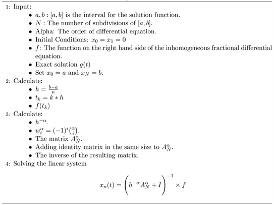
Algorithm 1. Numerical realization using matrix approach method.

For $N=60$ and $N=70$, Figure 2(a) and Figure 3(a) compare both the exact and numerical solutions for the fractional differential Equation (30). Moreover, Figure 2(b) and Figure 3(b) show the absolute error between exact and numerical solutions.

Example 2. Consider the linear fractional differential equation:

$D^{\alpha }x\left(t\right)+x\left(t\right)=1,\alpha \in \left(1,2\right)$ (37)

with initial conditions: $x\left(0\right)=0,x^{\prime }\left(0\right)=0$.

(a) (b)

Figure 2. A comparison between exact and approximate solutions by applying Algorithm 1 for Equation (30) with $N=60$. (a) A comparison between the exact and approximate solution in example (1); (b) Absolute error between exact and numerical solution in example (1).

(a) (b)

Figure 3. A comparison between exact and approximate solutions by applying Algorithm 1 for Equation (30) with $N=70$. (a) A comparison between the exact and approximate solution in example (1); (b) Absolute error between exact and numerical solution in example (1).

The exact solution of Equation (37) is:

$x\left(t\right)=t^{1.1}{E}_{1.1,2.1}\left(-t^{1.1}\right)$

Now, we implement the homotopy perturbation method to solve Equation (37).

In virtue of Equation (11), we can write Equation (37) in the homotopy form:

$D^{\alpha }x\left(t\right)+px\left(t\right)-1=0$ (38)

The solution of Equation (38) has the form:

$x\left(t\right)=x_0\left(t\right)+p{x}_1\left(t\right)+p^2{x}_2\left(t\right)+p^3{x}_3\left(t\right)+\cdots$ (39)

Substituting Equation (39) into Equation (38) and collecting terms with the same power of p, then we get:

$\{\begin{array}{l}{p}^0:D^{\alpha }{x}_0\left(t\right)=0\\ p^1:D^{\alpha }{x}_1=-x_0\left(t\right)+f\left(t\right)\\ p^2:D^{\alpha }{x}_2\left(t\right)=-x_1\left(t\right)\\ p^3:D^{\alpha }{x}_3\left(t\right)=-x_2\left(t\right)\\ ⋮\end{array}$ (40)

Applying ${\Omega }^{\alpha }$ and the inverse operator of $D^{\alpha }$, on both sides of Equation (40), then we get: and using the definition of Riemann-Liouville fractional integral operator ( ${\Omega }^{\alpha }$ ) of order $\alpha \ge 0$ we obtain:

$\begin{array}{c}{x}_0\left(t\right)={\displaystyle \underset{i=0}{\overset{1}{\sum }}}{x}^{\left(i\right)}\left(0\right)\frac{t^i}{i!}\\ =x\left(0\right)\frac{t^0}{0!}+x^{\prime }\left(0\right)\frac{t^1}{1!}\\ =0\end{array}$

$\begin{array}{c}{x}_1\left(t\right)=-{\Omega }^{\alpha }\left[x_0\left(t\right)+{\Omega }^{\alpha }\left[f\left(t\right)\right]\right]\\ ={\Omega }^{\alpha }\left[1\right]\\ =\frac{t^{\alpha }}{\Gamma \left(1+\alpha \right)}\end{array}$

$\begin{array}{c}{x}_2\left(t\right)=-{\Omega }^{\alpha }\left[x_1\left(t\right)\right]\\ =-{\Omega }^{\alpha }\left[\frac{t^{\alpha }}{\Gamma \left(1+\alpha \right)}\right]\\ =-\frac{t^{2\alpha }}{\Gamma \left(2\alpha +1\right)}\end{array}$

$\begin{array}{c}{x}_3\left(t\right)=-{\Omega }^{\alpha }\left[x_2\left(t\right)\right]\\ =-{\Omega }^{\alpha }\left[-\frac{t^{2\alpha }}{\Gamma \left(2\alpha +1\right)}\right]\\ =\frac{t^{3\alpha }}{\Gamma \left(3\alpha +1\right)}\end{array}$

$⋮$

Then the solution of Equation (37) has the general form:

$x\left(t\right)=x_0\left(t\right)+x_1\left(t\right)+x_2\left(t\right)+x_3\left(t\right)+\cdots$ (41)

$x\left(t\right)=\frac{t^{\alpha }}{\Gamma \left(1+\alpha \right)}-\frac{t^{2\alpha }}{\Gamma \left(2\alpha +1\right)}+\frac{t^{3\alpha }}{\Gamma \left(3\alpha +1\right)}+\cdots$ (42)

$x\left(t\right)={\displaystyle \underset{i=1}{\overset{\infty }{\sum }}}{\left(-1\right)}^{i+1}\left(0\right)\frac{t^{\alpha i}}{\Gamma \left(\alpha i+1\right)}$ (43)

when $\alpha =1.1$, we get

$\begin{array}{c}x\left(t\right)=\frac{t^{1.1}}{\Gamma \left(2.1\right)}-\frac{t^{2.2}}{\Gamma \left(3.2\right)}-\frac{t^{3.3}}{\Gamma \left(4.3\right)}-\frac{t^{4.4}}{\Gamma \left(5.4\right)}+\cdots \\ =\frac{t^{1.1}}{0.95135}-\frac{t^{2.2}}{0.95135}-\frac{t^{3.3}}{0.95135}-\frac{t^{4.4}}{0.95135}+\cdots \\ =0.95557t^{1.1}-0.41255t^{2.2}+0.11293t^{3.3}-0.02242t^{4.4}+\cdots \end{array}$ (44)

Now, we implement Algorithm 1 to solve Equation (37) using the matrix approach method. Table 2 contains the exact and numerical results using the matrix approach method with $\alpha =1.1$ and $N=51$. The maximum error with $N=51$ is 0.015888820145463. Figure 4(a) compares both the exact and numerical solutions for the (37). Moreover, Figure 4(b) shows the absolute error between exact and numerical solutions. For $N=60$ and $N=70$, Figure 5(a) and Figure 6(a) compare both the exact and numerical solutions for the fractional differential Equation (30). Moreover, Figure 5(b) and Figure 6(b) show the absolute error between exact and numerical solutions.

Table 2. The exact and numerical solutions using the matrix approach method where $N=51$.

(a) (b)

Figure 4. A comparison between exact and approximate solutions by applying Algorithm 1 for Equation (37) with $N=51$. (a) A comparison between the exact and approximate solution in example (2); (b) Absolute error between exact and numerical solution in example (2).

(a) (b)

Figure 5. A comparison between exact and approximate solutions by applying Algorithm 1 for Equation (37) with $N=60$. (a) A comparison between the exact and approximate solution in example (2); (b) Absolute error between exact and numerical solution in example (2).

(a) (b)

Figure 6. A comparison between exact and approximate solutions by applying Algorithm 1 for Equation (37) with $N=70$. (a) A comparison between the exact and approximate solution in example (2); (b) Absolute error between exact and numerical solution in example (2).

6. Conclusion

In this article, two numerical techniques namely, the homotopy perturbation method and the matrix approach method have been proposed and implemented to solve fractional differential equations. The accuracy and the validity of these techniques are tested with some numerical examples. The results show clearly that both techniques are in a good agreement with the analytical solution. According to numerical results mentioned in tables and figures, we conclude that the matrix approach method provides more accurate results than its counterpart and therefore is more advantageous. In addition, we strongly believe that the matrix approach method is regarded to be one of the most effective methods among the other methods mentioned in the literature. It is known for its fast converges and accuracy.

List of Nomenclatures

1) $D^{\alpha }$ : Fractional Derivative.

2) $\Gamma \left(p\right)$ : Gamma Function.

3) $\Omega$ : Libera Integral Operator.

4) ${\Omega }^{\alpha }$ : Riemann-Liouville Fractional Integral Operator.

5) $\left\{{\sin }_{\alpha }{t}^{\alpha }\mathrm{,}{\cos }_{\alpha }{t}^{\alpha }\mathrm{,}{\sinh }_{\alpha }{t}^{\alpha }\mathrm{,}{\cosh }_{\alpha }{t}^{\alpha }\right\}$ : Mittage Leffer Functions.

6) $j^0$ : Identity Operator.

7) ${}_{d}D{}_t^p$ : Grumwald-Letnikov Fractional Derivative.

8) $D_{\mathrm{0,}t}^p$ : Riemann-Liouville Derivative of Order p.

9) $D_{\ast }^{\alpha }$ : Caputo Fractional Derivative.

Conflicts of Interest

The authors declare that they have no conflict of interest.

References

[1]	Carpinteri, A. and Mainardi, F. (2014) Fractals and Fractional Calculus in Continuum Mechanics. Springer, Berlin.
[2]	Wazwaz, A.-M. (2011) Linear and Nonlinear Integral Equations. Springer, Berlin. https://doi.org/10.1007/978-3-642-21449-3
[3]	Agarwal, R., Jain, S. and Agarwal, R.P. (2015) Solution of Fractional Volterra Integral Equation and Non-Homogeneous Time Fractional Heat Equation Using Integral Transform of Pathway Type. Progress in Fractional Differentiation and Applications, 1, 145-155.
[4]	Bandrowski, B., Karczewska, A. and Rozmej, P. (2010) Numerical Solutions to Integral Equations Equivalent to Differential Equations with Fractional Time. International Journal of Applied Mathematics and Computer Science, 20, 261-269. https://doi.org/10.2478/v10006-010-0019-1
[5]	Metzler, R., Schick, W., Kilian, H.-G. and Nonnenmacher, T.F. (1995) Relaxation in Filled Polymers: A Fractional Calculus Approach. The Journal of Chemical Physics, 103, 7180-7186. https://doi.org/10.1063/1.470346
[6]	Oldham, K. and Spanier, J. (1974) The Fractional Calculus Theory and Applications of Differentiation and Integration to Arbitrary Order. Elsevier, Amsterdam.
[7]	Srivastava, T., Singh, A.P. and Agarwal, H. (2015) Modeling the Under-Actuated Mechanical System with Fractional Order Derivative. Progress in Fractional Differentiation and Applications, 1, 57-64.
[8]	Sharma, M., Ali, M.F. and Jain, R. (2015) Advanced Generalized Fractional Kinetic Equation in Astrophysics. Progress in Fractional Differentiation and Applications, 1, 65-71.
[9]	Caputo, M. (1967) Linear Models of Dissipation Whose Q Is Almost Frequency Independent? II. Geophysical Journal International, 13, 529-539. https://doi.org/10.1111/j.1365-246X.1967.tb02303.x
[10]	Kolwankar, K.M. and Gangal, A.D. (1996) Fractional Differentiability of Nowhere Differentiable Functions and Dimensions. Chaos: An Interdisciplinary Journal of Nonlinear Science, 6, 505-513. https://doi.org/10.1063/1.166197
[11]	Liu, Z.H. and Liang, J.T. (2013) A Class of Boundary Value Problems for First-Order Impulsive Integro-Differential Equations with Deviating Arguments. Journal of Computational and Applied Mathematics, 237, 477-486. https://doi.org/10.1016/j.cam.2012.06.018
[12]	Liu, Z.H., Sun, J.H. and Szántó, I. (2013) Monotone Iterative Technique for Riemann-Liouville Fractional Integro-Differential Equations with Advanced Arguments. Results in Mathematics, 63, 1277-1287. https://doi.org/10.1007/s00025-012-0268-4
[13]	Liu, Z.H., Loi, N. and Obukhovskii, V. (2013) Existence and Global Bifurcation of Periodic Solutions to a Class of Differential Variational Inequalities. International Journal of Bifurcation and Chaos, 23, Article ID: 1350125. https://doi.org/10.1142/S0218127413501253
[14]	Liu, Z.H., Lu, L. and Szántó, I. (2013) Existence of Solutions for Fractional Impulsive Differential Equations with p-Laplacian Operator. Acta Mathematica Hungarica, 141, 203-219. https://doi.org/10.1007/s10474-013-0305-0
[15]	Liu, X.Y. and Liu, Z.H. (2013) Existence Results for a Class of Second Order Evolution Inclusions and Its Corresponding First Order Evolution Inclusions. Israel Journal of Mathematics, 194, 723-743. https://doi.org/10.1007/s11856-012-0092-2
[16]	Qu, H.D. and Liu, X. (2013) Existence of Nonnegative Solutions for a Fractional m-Point Boundary Value Problem at Resonance. Boundary Value Problems, 213, 127. https://doi.org/10.1186/1687-2770-2013-127
[17]	Odibat, Z., Momani, S. and Xu, H. (2010) A Reliable Algorithm of Homotopy Analysis Method for Solving Nonlinear Fractional Differential Equations. Applied Mathematical Modelling, 34, 593-600. https://doi.org/10.1016/j.apm.2009.06.025
[18]	Das, S. and Gupta, P.K. (2011) Homotopy Analysis Method for Solving Fractional Hyperbolic Partial Differential Equations. International Journal of Computer Mathematics, 88, 578-588. https://doi.org/10.1080/00207161003631901
[19]	Elsaid, A. (2011) Homotopy Analysis Method for Solving a Class of Fractional Partial Differential Equations. Communications in Nonlinear Science and Numerical Simulation, 16, 3655-3664. https://doi.org/10.1016/j.cnsns.2010.12.040
[20]	Chandel, R.S., Singh, A. and Chouhan, D. (2017) Numerical Solution of Fractional Order Differential Equations Using Haar Wavelet Operational Matrix. Palestine Journal of Mathematics, 6, 515-3523.
[21]	Qu, H.D. and Liu, X. (2015) A Numerical Method for Solving Fractional Differential Equations by Using Neural Network. Advances in Mathematical Physics, 2015, Article ID: 439526. https://doi.org/10.1155/2015/439526
[22]	Hamdan, S., Qatanani, N. and Daraghmeh, A. (2019) Numerical Techniques for Solving Linear Volterra Fractional Integral Equation. Journal of Applied Mathematics, 2019, Article ID: 5678103. https://doi.org/10.1155/2019/5678103
[23]	Saadeh, A. (2018) Numerical Methods for Solving Fractional Differential Equations with Applications. An-Najah National University MSc Thesis.
[24]	Lee, T.-D., Oehme, R. and Yang, C.-N. (1957) Remarks on Possible Noninvariance under Time Reversal and Charge Conjugation. Physical Review, 106, 340. https://doi.org/10.1103/PhysRev.106.340
[25]	Gorenflo, R., Mainardi, F. and Podlubny, I. (1999) Fractional Differential Equations. Academic Press, Cambridge, 683-699.
[26]	Miller, K.S. and Ross, B. (1993) An Introduction to the Fractional Calculus and Fractional Differential Equations. John-Wily and Sons Inc., New York.
[27]	Mainardi, F. (1997) Fractional Calculus. In: Fractals and Fractional Calculus in Continuum Mechanics, Springer, Berlin, 291-348. https://doi.org/10.1007/978-3-7091-2664-6_7
[28]	Courant, R. (1966) Methods of Mathematical Physics, Volume II: Partial Differential Equations. Interscience Publishers Inc., New York.
[29]	Ishteva, M. (2005) Properties and Applications of the Caputo Fractional Operator. Department of Mathematics, University of Karlsruhe, Karlsruhe.